Out of all the apps on my phone, the camera is one that I can't see myself without anymore. Between being out with friends, or travelling with family, the camera rarely remains idle as I capture memories forever. Though, there is one particular feature of mobile photography I've come to especially love: the panorama.

Even this struggles to capture how well the Grand Canyon lives up to its name.
Something about the extreme wide angle capturing more than what your eye can behold all at once makes it truly magical. And, if you have an Android phone, you can get even more incredible types of otherwise impossible photos with Google's staple Photo Spheres:
An "unwrapped" Photo Sphere; normally this would be an interactive literal sphere of the environment.
While these are cool, it does beg the question: how are these made? It's not like your phone is able to take them in a single snapshot; usually you have to spin or take multiple photos. How is your phone able to tie multiple images together into a single cohesive one? We'll explore a little bit of linear algebra to manipulate our photos exactly how we want to, and indulge in stylistic photos your others can only dream of.
The Problem
Before anything else, let's first define what a panorama is. In computer graphics, a panorama is a type of mosaic, that is, a unification of two or more images. A panorama in particular, though, is a mosaic in which all the photos to be stitched together are all taken from the same camera position. When you take a panorama on your phone, all you're doing is spinning in place, so that's what we want to recreate.
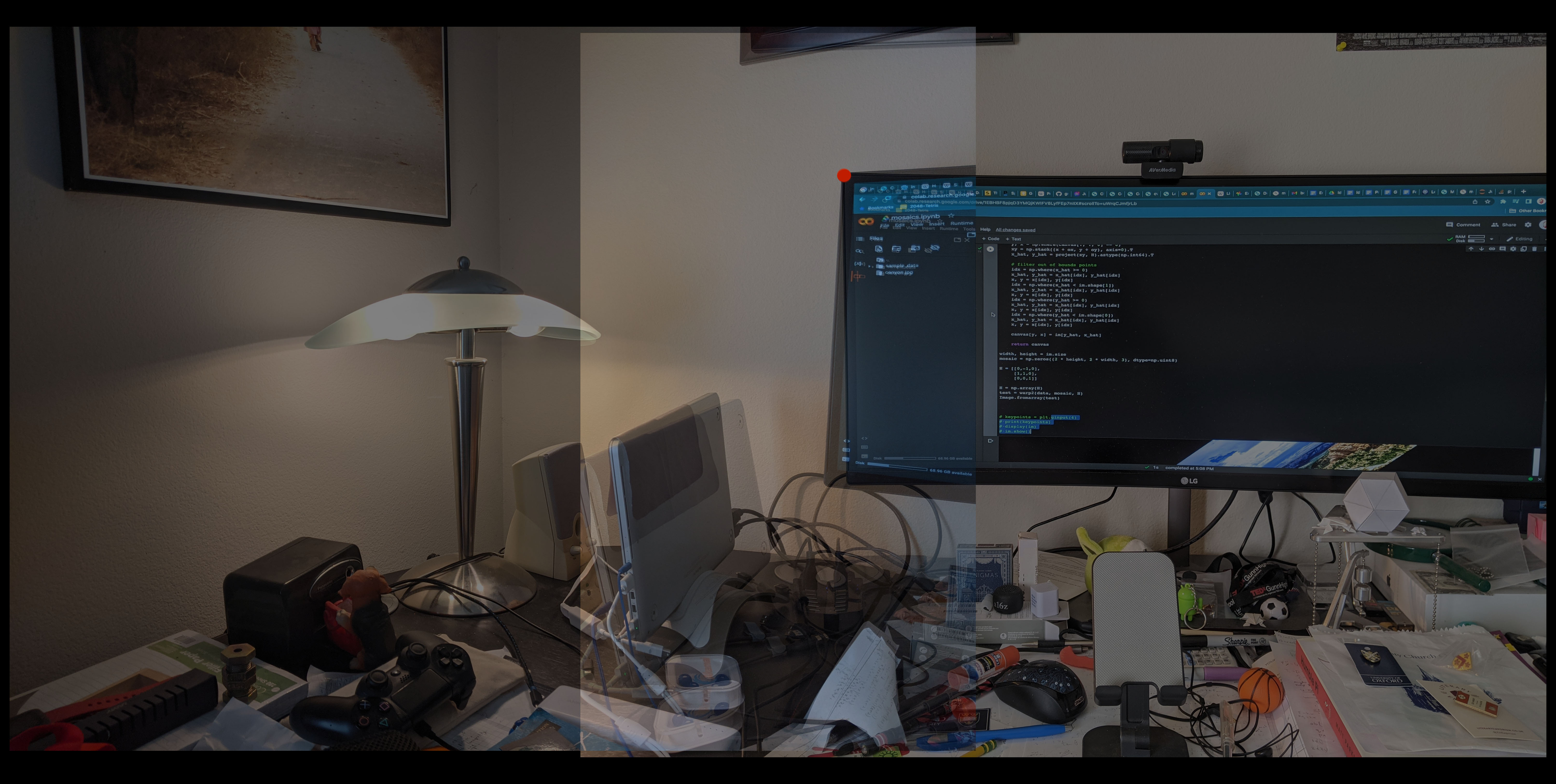
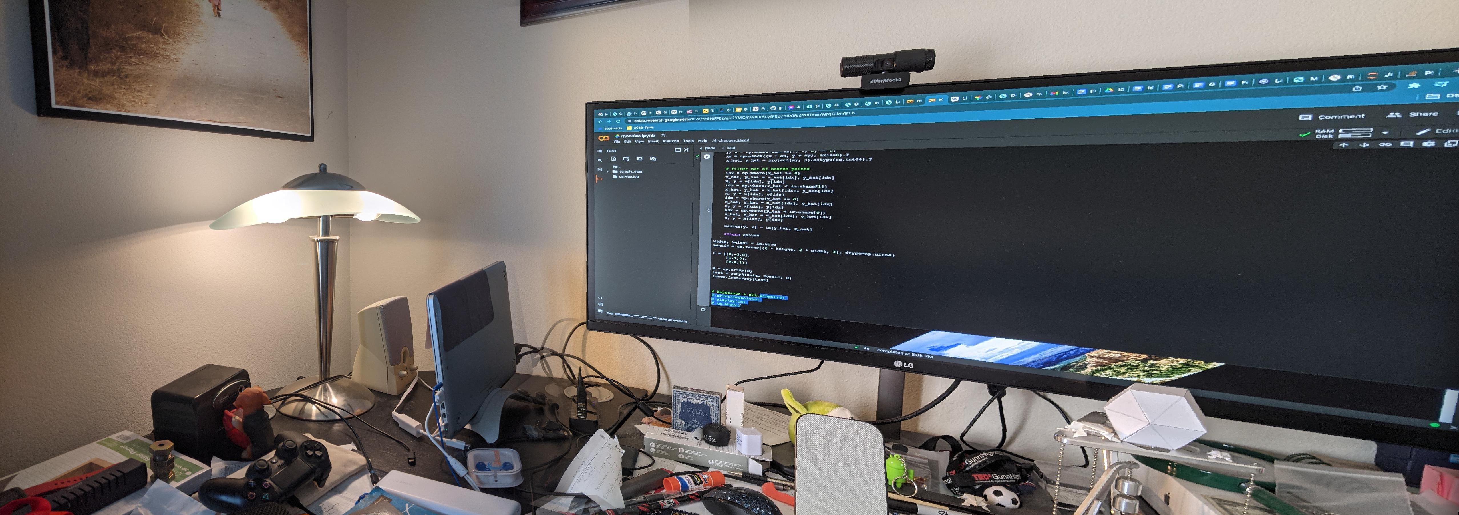
So, if we're given two images from different angles,

how do we combine them into a single unified image? Thinking about it this way is not super helpful, since, well, that's what we already know about panoramas. What do we want to get out of a panorama? If our panorama is done well, then objects in one image should overlap properly with the same objects in the other image.
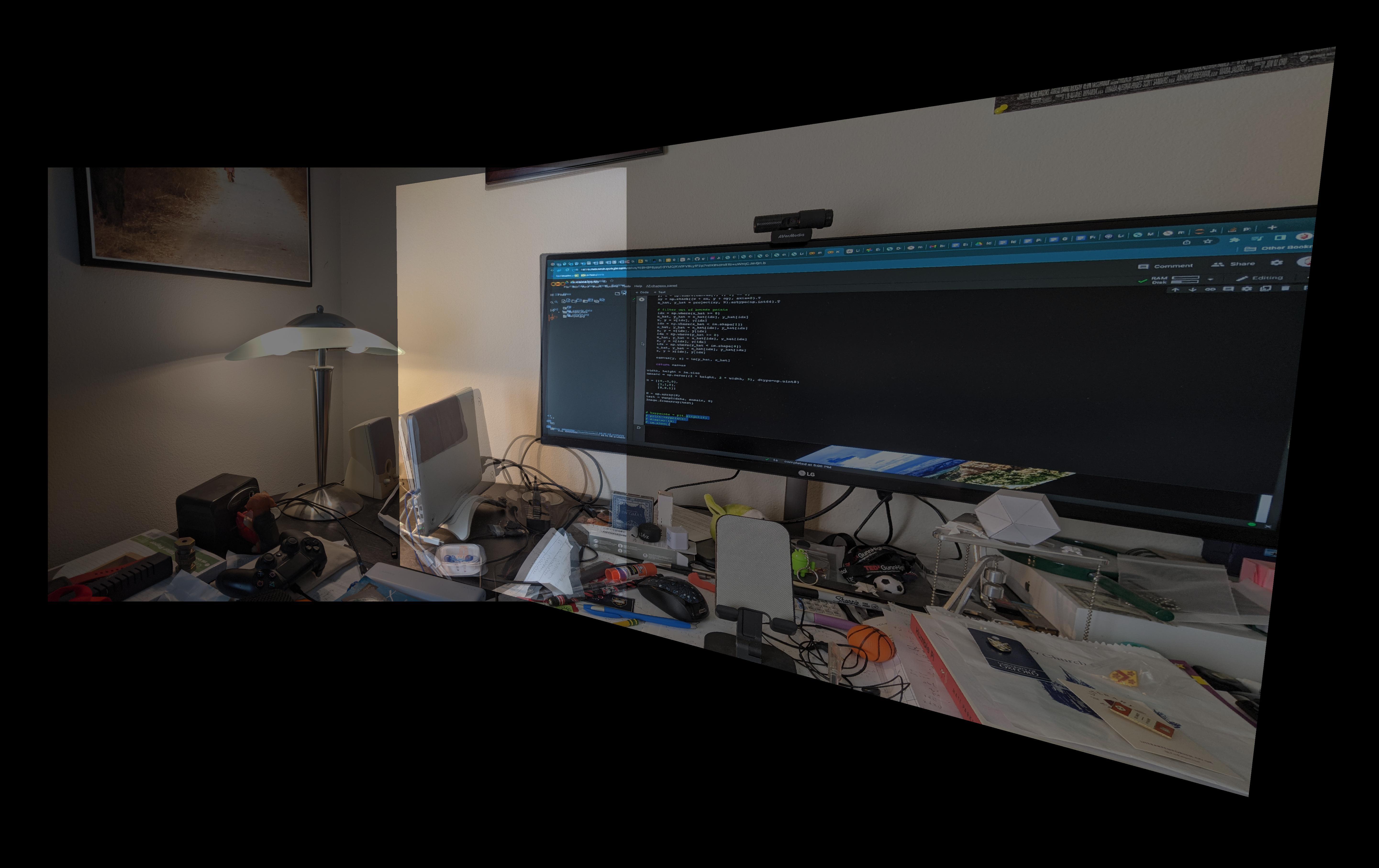
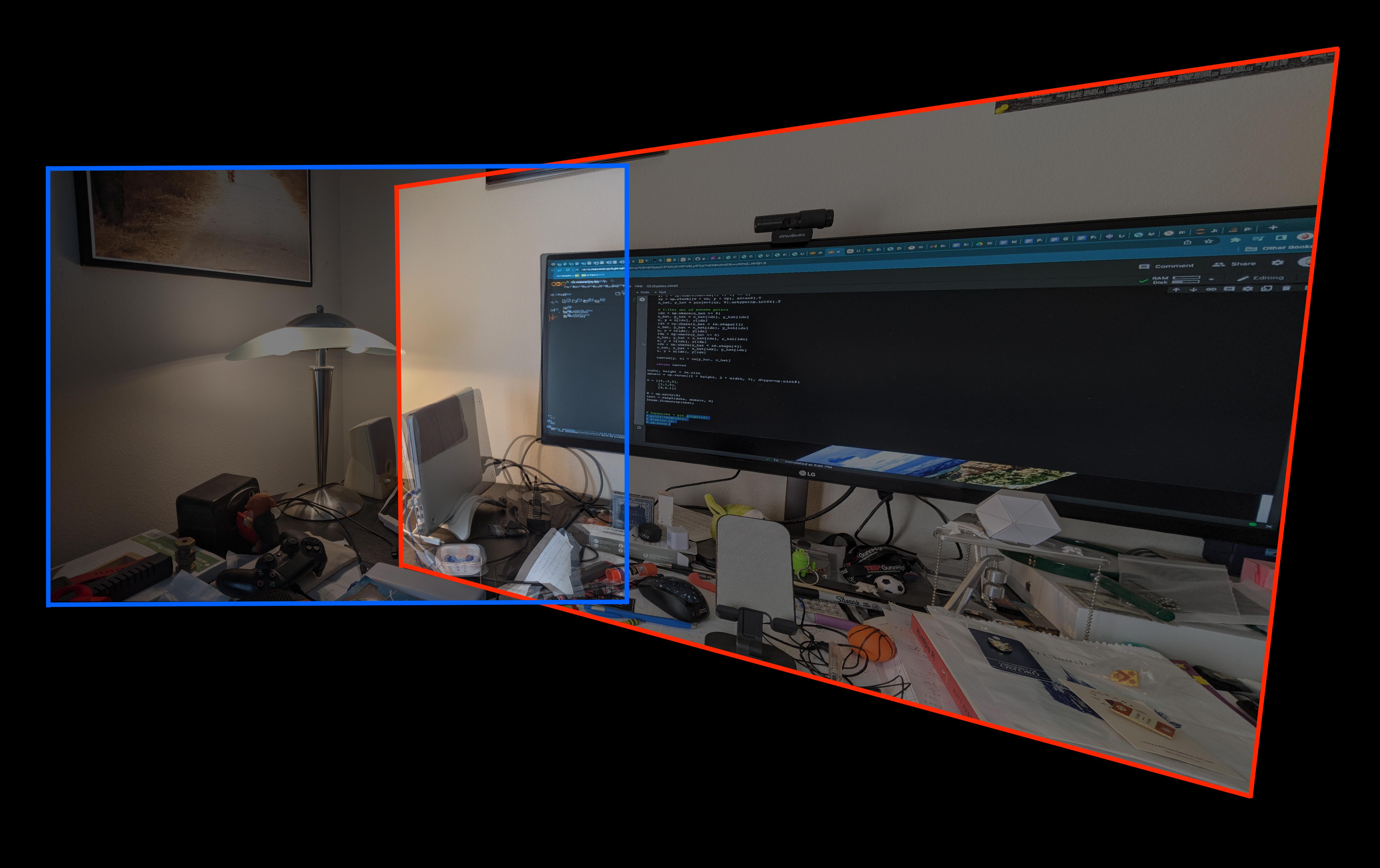
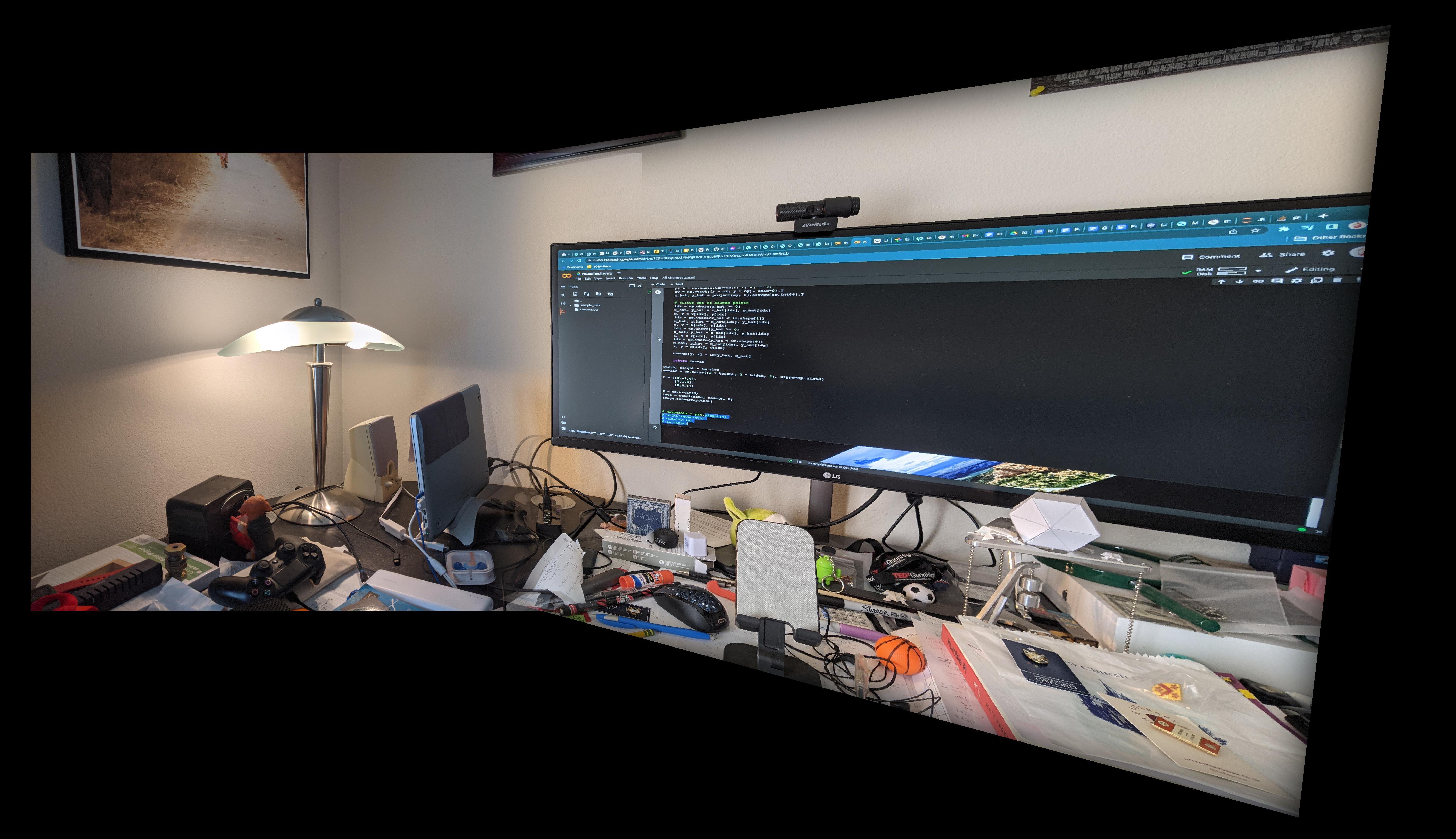
For example, take a look at the top left of my computer monitor:
In our panorama, these two points should overlap, since we obviously recognize these to be the same object in the real world. But to the two pictures, they are wildly different! In the first picture, the corner of my monitor is closer to the left side of the frame, while in the second picture, it is almost on the top-right edge of the image. So, if we try to manually align these two corners so that they overlap, we get:
While our single corner of the monitor is aligned between the two images, I don't think I have to try very hard to convince you that this isn't a great panorama. I mean, just look at the rest of the overlap.
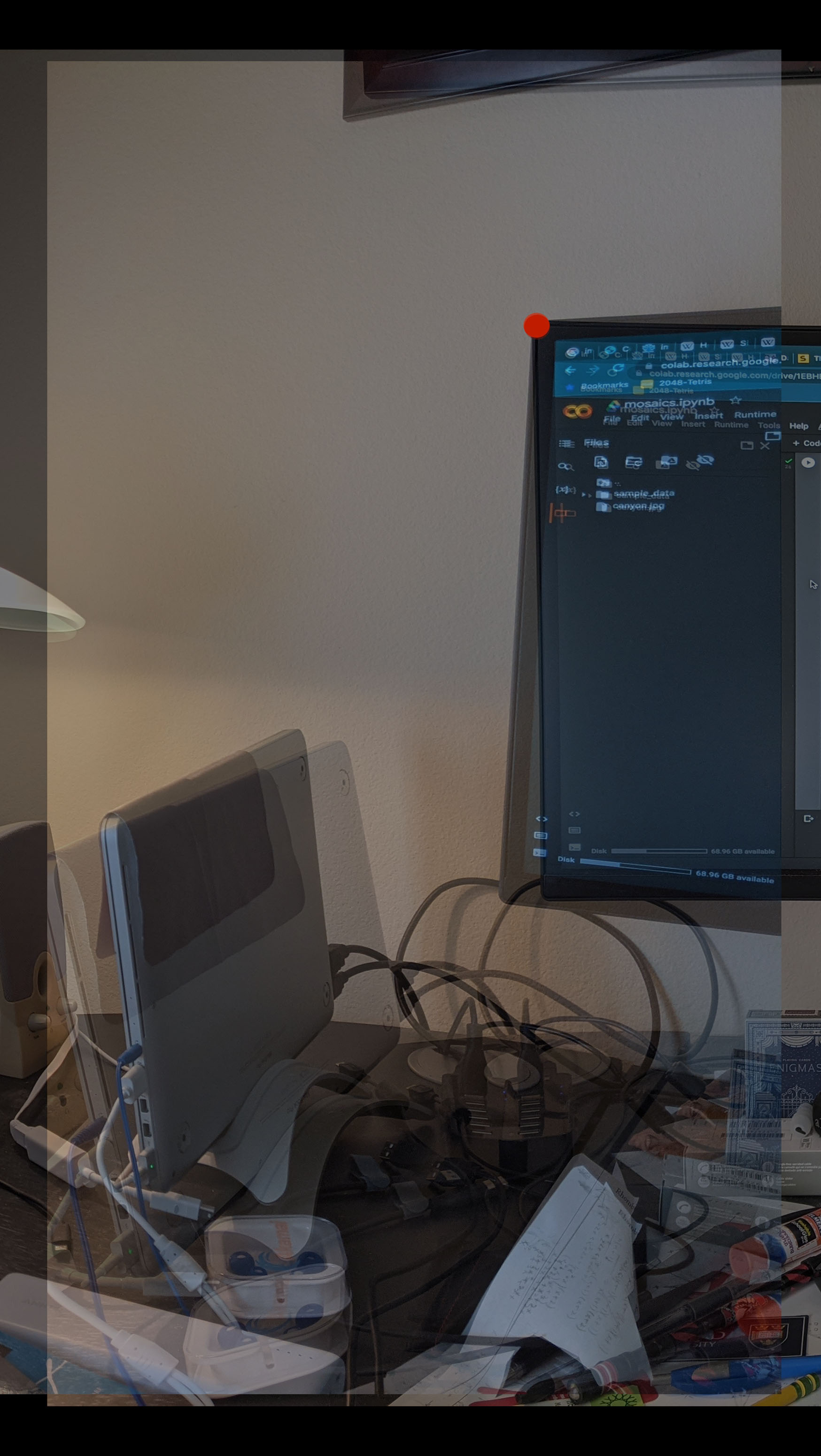
The skew angles of the resting laptop and the monitor itself don't align at all, and while my cable management is bad, it's not that bad. This is the real challenge at the heart of making panoramas: images are flat, while the motion of a panorama is cylindrical. Ideally we would take a "cylindrical" photo and unwrap that into a rectangle, but we can't. Undoubtedly, we will have to warp our images somehow to align.
How do we find the right way to warp our image? The first thing we will need to do is get more data! Having one point line up between the photos is not great, but, say, 10 different data points might not be bad.
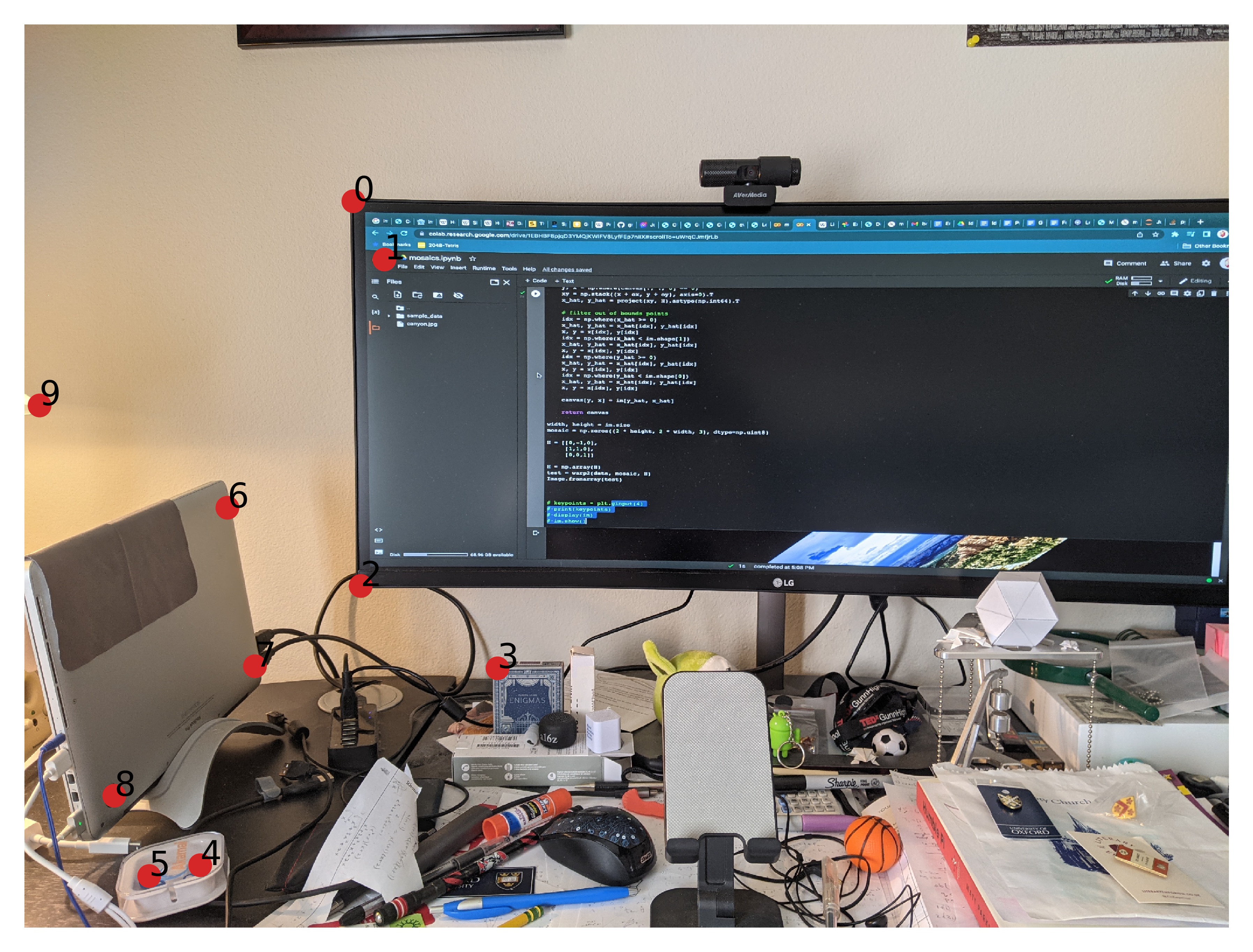
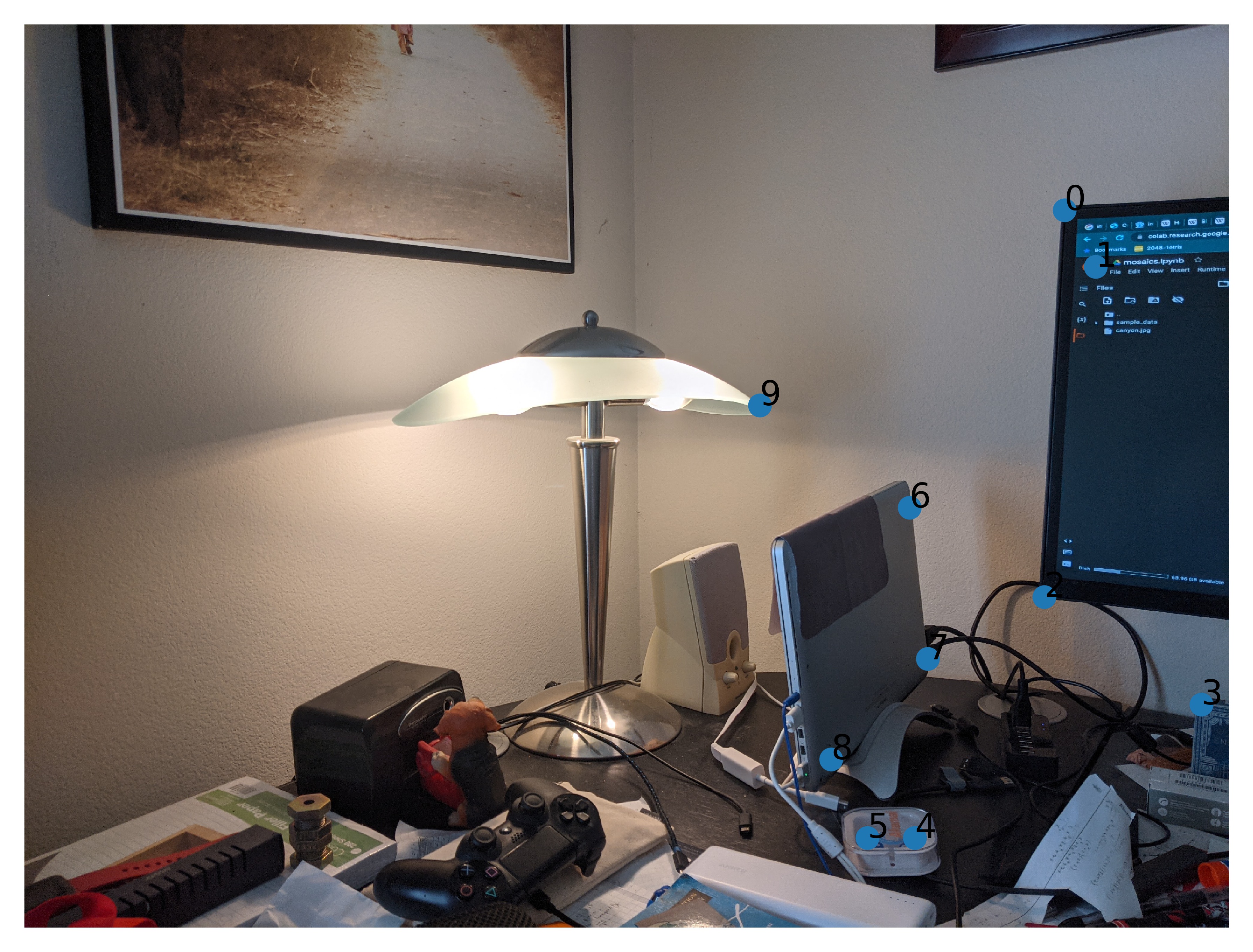
So, our final panorama would like the same numbered red and blue points to overlap. With data to use, the second thing we will need is a way to actually warp our image; how do we actually make our points between photos line up? For that, we turn to linear algebra.
Rethinking Coordinates
If you had a random ordinary point, how might you describe its position to someone?
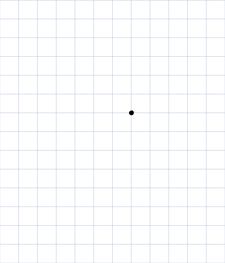
A lonely, solitary point living in the plane.
A common choice we're all familiar with in some way is by using a coordinate system. That is, we define a place to be $(0,0)$ and locate every point relative to that origin in terms of its $x$ and $y$ coordinates $(x,y)$.
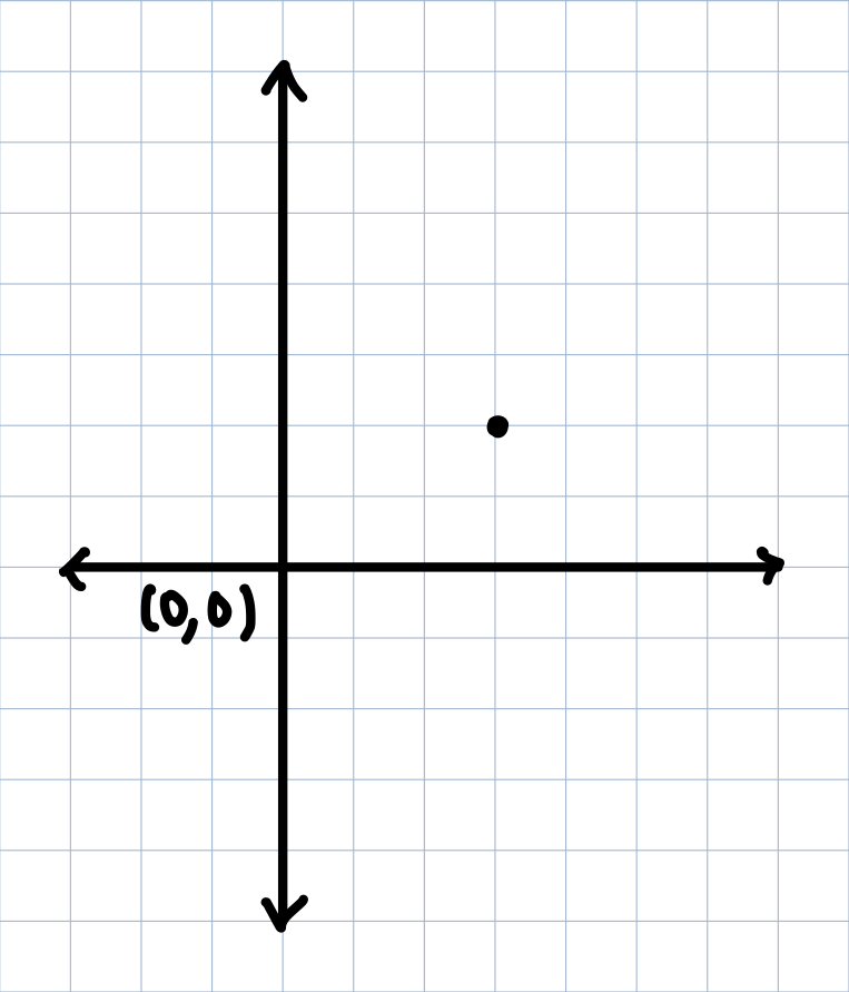
A still lonely, solitary point living in the plane, but with more lines.
In the above coordiante space choice, we might say the point is at $(3,2)$. But what exactly do we mean by the point being at $(3,2)$? What this really implies is that the point is 3 steps to the right of the origin, and 2 steps above the origin.
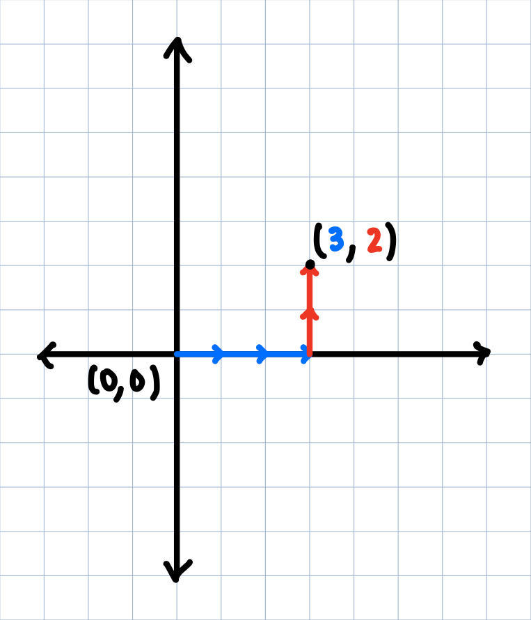
So, instead of thinking of this point in terms of separate coordinates, we can think of it in terms of these two basis vectors. Let's use $\color{blue}{i}$ to represent the blue, horizontal vector, and $\color{red}{j}$ to represent the red, vertical vector. So, our point is really the combination of $\color{blue}{3i}$ and $\color{red}{2j}$, or simply, $\color{blue}{3i} + \color{red}{2j}$, which itself repsents another vector (the one pointing from the origin to the point $(3,2)$).
This might seem extra and unnecessary, since we just rewrote a vector as the sum of its horizontal and vertical components, which is what coordinates literally do in the first place. But the useful insight here is that there is nothing that says our basis vectors have to be in the unit directions! We can now rewrite points in multiple ways depending on our choice of $\color{blue}{i}$ and $\color{red}{j}$.
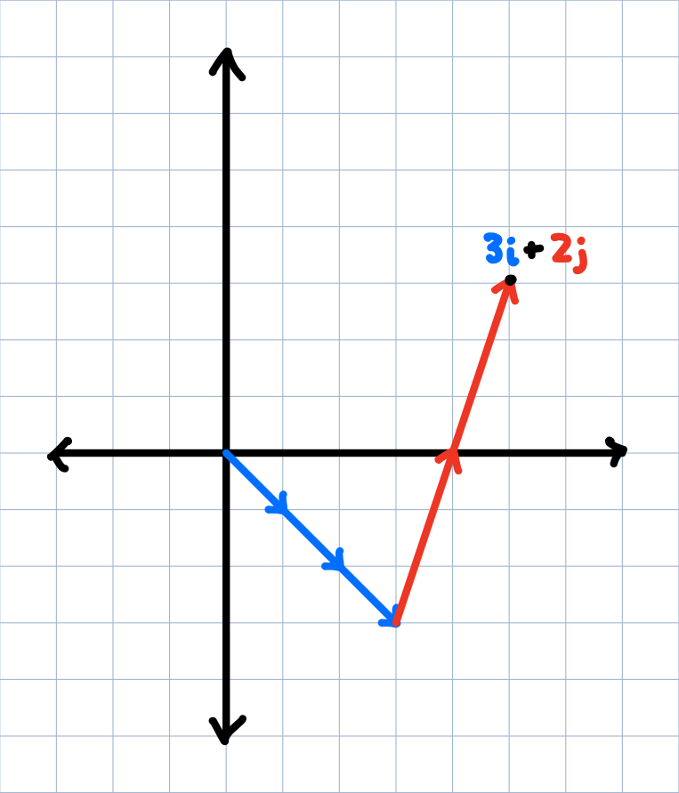
A new, quirky choice of basis vectors.
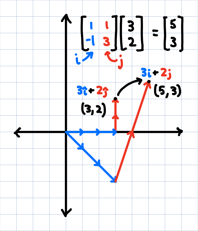
With a new choice of basis vectors, the vector $\color{blue}{3i} + \color{red}{2j}$ has a totally new position as that now encodes the coordinate $(5,3)$ since neither $\color{blue}{i}$ nor $\color{red}{j}$ represents horizontal or vertical steps anymore, but rather skew, diagonal steps.
But look at that! We've basically accomplished our goal of warping points! We've managed to transform the point $(3,2) \rightarrow (5,3)$ by manipulating $\color{blue}{i}$ and $\color{red}{j}$; both points are techincally at $\color{blue}{3i} + \color{red}{2j}$, just for different basis vectors.
This is what linear algebra and matrices encode geometrically. If we write our basis vectors $\color{blue}{i}$ and $\color{red}{j}$ in a matrix and multiply that by the vector representing our initial point, we will get a new point representing our transformation (a.k.a., our warp). How do we write our basis vectors in a matrix? Each vector implicitly has coordinates associated with themselves! In the above picture, $\color{blue}{i}$ points at $\color{blue}{(1,-1)}$, since from its tail to its tip it moves one step to the right and one step down. $\color{red}{j}$, on the other hand, points at $\color{red}{(1,3)}$, and these are precisely the vectors we see in our matrix.
For the unit basis vectors that point at $(1,0)$ and $(0,1)$, to differentiate them from any old pair of basis vectors, we call them $\color{blue}{\hat{\imath}}$ and $\color{red}{\hat{\jmath}}$ wearing a little hat, and their respective matrix the identity matrix, since it leaves vectors unchanged after multiplication (since that's what we used to define coordinates in the first place).
The underlying idea of linear transformations.
These $2 \times 2$ matrices represent linear transformations. They're transformations in they way that they transform points from one coordinate to another (well, most of them at least), and they are linear in the sense that keep all grid lines parallel, evenly spaced and, well, linear after the transformation. This is best seen through video and not stills. For this post you don't need to understand the mechanics of matrix-vector multiplication, but just understand that it represents some transformation on a point.
Warping Images
So why should we care? Why is this helpful in any way? If we think of each pixel on our images as a coordinate, we can just apply our transformation to all pixels on that image, find where they land and color them, and generate a new image. Let's take this picture as an example.

We can scale it, rotate it, or even shear it by applying the same transformation matrix to every pixel by changing $\color{blue}{i}$ and $\color{red}{j}$ like before.
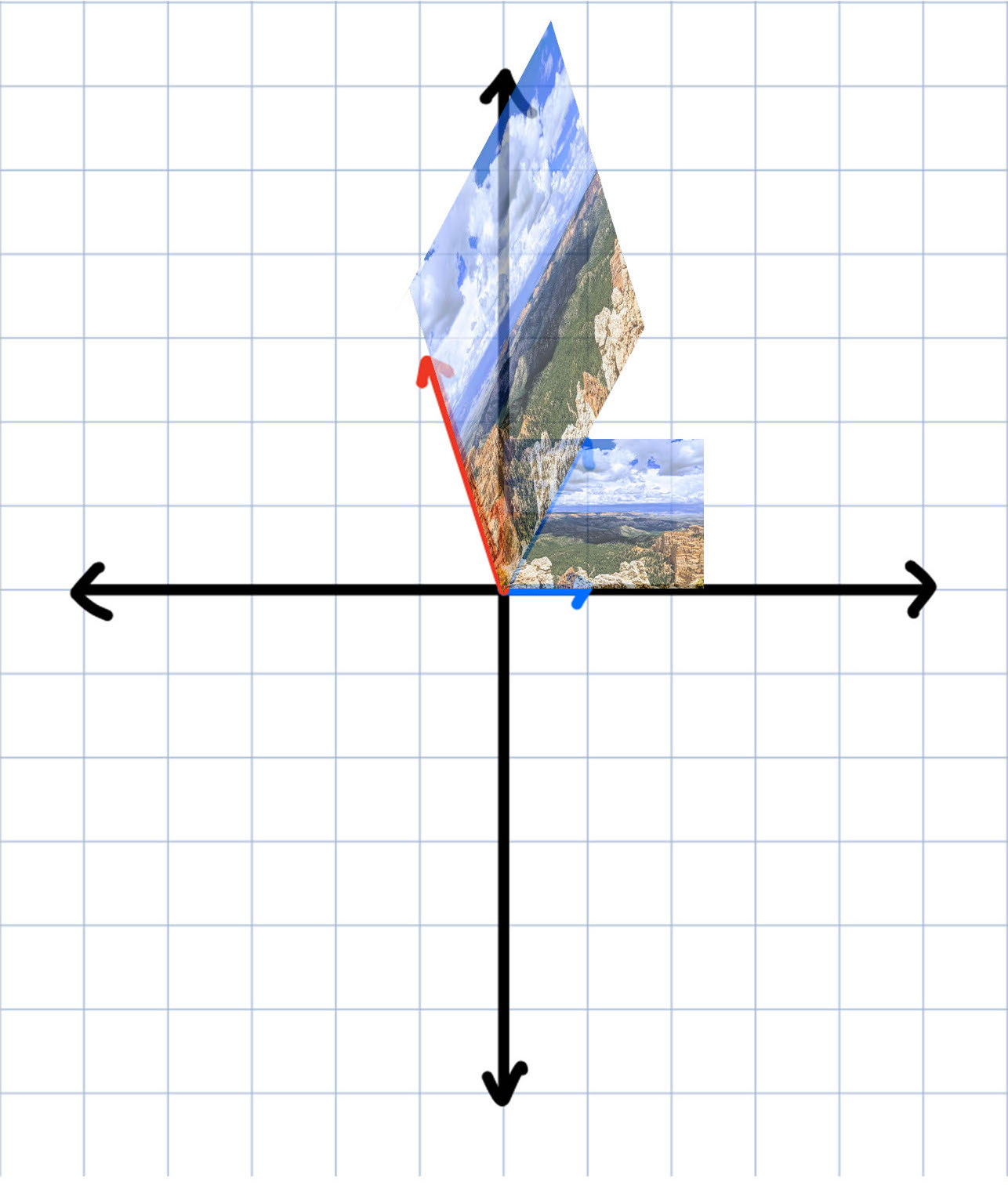
An example transformation acting on our image.
But we have a big problem here: the typical linear transformation does not allow for translations. By the qualities of linear transformations, the origin cannot move, therefore forcing the bottom left corner of our images to always overlap! That's pretty restrictive in terms of the panoramas we can make—and for practical purposes—a complete nonstarter. If we want to continue through with making a panorama, we'll need to find a way around translations.
Homogenous Coordinates and Affine Transformations
There's a very sneaky workaround being confined to the origin. To do so, we'll need to do something that might seem a bit weird to do translations. Let's rewrite our 2D points with a 3rd coordinate. For a given $(x,y)$, let's rewrite that with a $z$-coordinate $(x,y,1)$. If $z \neq 1$, then we can just divide all the other coordinates by $z$ to make it equal to 1: $(x,y,w) \rightarrow (\frac{x}{w}, \frac{y}{w}, 1)$ (we generally use $w$ to represent the $z$-coordinate to indicate that there is no "real" $z$ value since everything is projected into 2D; we use $w$ as a "weight" to say how much we scale our projections down to). This means we have multiple coordinates represent the same point. In this way, $(2,5,1)$ and $(4,10,2)$ and $(-3,-7.5,-1.5)$ and $(2w,5w,w)$ all represent the same point (we don't include points when $z=0$ as it represents a point at infinity).
This might seem arbitrary, but what we're doing here is not too different than our original, 2-coordinate system. When we look at a cross-section of the $xyz$ coordinate space, it looks exactly like the $xy$ plane. What we are doing here is projecting all of $xyz$ space onto the plane $z=1$.
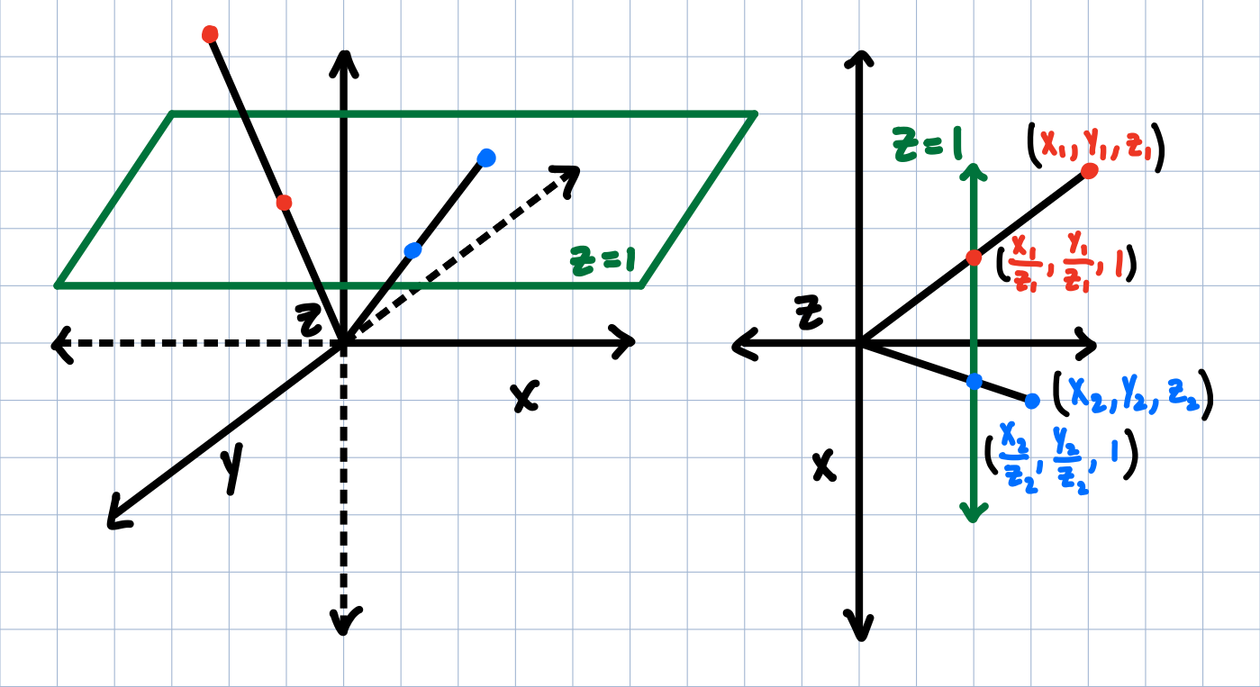
The geometry of projecting points onto $z=1$ is equivalent to drawing a line through the origin and the point, and finding where it intersects that plane.
In fact, many of you are already familiar with homogeneous coordinates (representing 2D points with a 3rd scalar coordinate) and projective planes! When you take a photo on your phone, how does the camera know what's drawn in its frame? How does it take a 3-dimensional world and put it into a 2-dimensional picture? The many light rays that enter the camera lens (the origin) will intersect a plane ($z=1$) based on its focal length, and colors the pixel based on the projection.
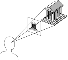
A photo is homogeneous coordinates in disguise. While there's many sides to the building, our camera only cares about what it sees in front of it (a.k.a., what gets projected onto the frame). Our worldview is contained to a small projection.
Using this analogy with photos, clearly translations should be possible! If you've seen any cat videos on the internet, clearly it is possible for the cat to enter and exit the frame freely without the camera necessarily moving, and that is precisely possible due to the fact the origin $(0,0,0)$ is not contained in our projective plane $z=1$, since all of our basis vectors have to stem out of the origin! (For those interested a translation matrix is equivalent to a shear along the $z$-axis.)
Think about what we're doing here: we're turning a linear transformation in 3-dimensions to create special non-linear affine transformations in 2-dimensions! When I first learned this geometrically, awe can't encapsulate the total shock I felt. So, if we're given a point $p$, we can transform it with a matrix $M$ to get its image $p'$.
(Notice how $M$ is now a $3 \times 3$ matrix as we are working with 3D coordinates now) If our matrix-vector product results in a $w$ value not equal to 1, then we just divide everything by $w$ to make it so, and get our coordinate in terms of our 2D plane.
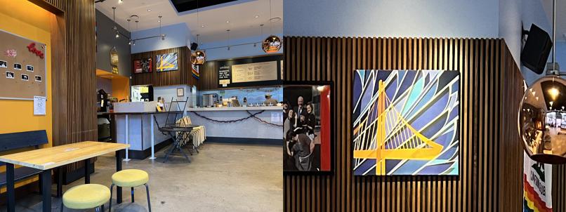
These projections with homogeneous coordinates are known as homographies. When we take one picture, and reproject it according to a matrix like this but keeping the same camera center (like the origin), we call it a homography. Again, like homogeneous coordinates, people have been leveraging homographies for a while now. You know how on roads, whenever there's text written like, "STOP AHEAD", it's always a bit vertically stretched? That's because when you read it at the angle of a driver in a car, it looks more regular and readable. At least, that's my theory.
More creatively, that weird, perspective street art you might have seen before? That's the most manual you can get to using homographies—literally warping images with the angle you look at them to make them appear at a normal proportion.
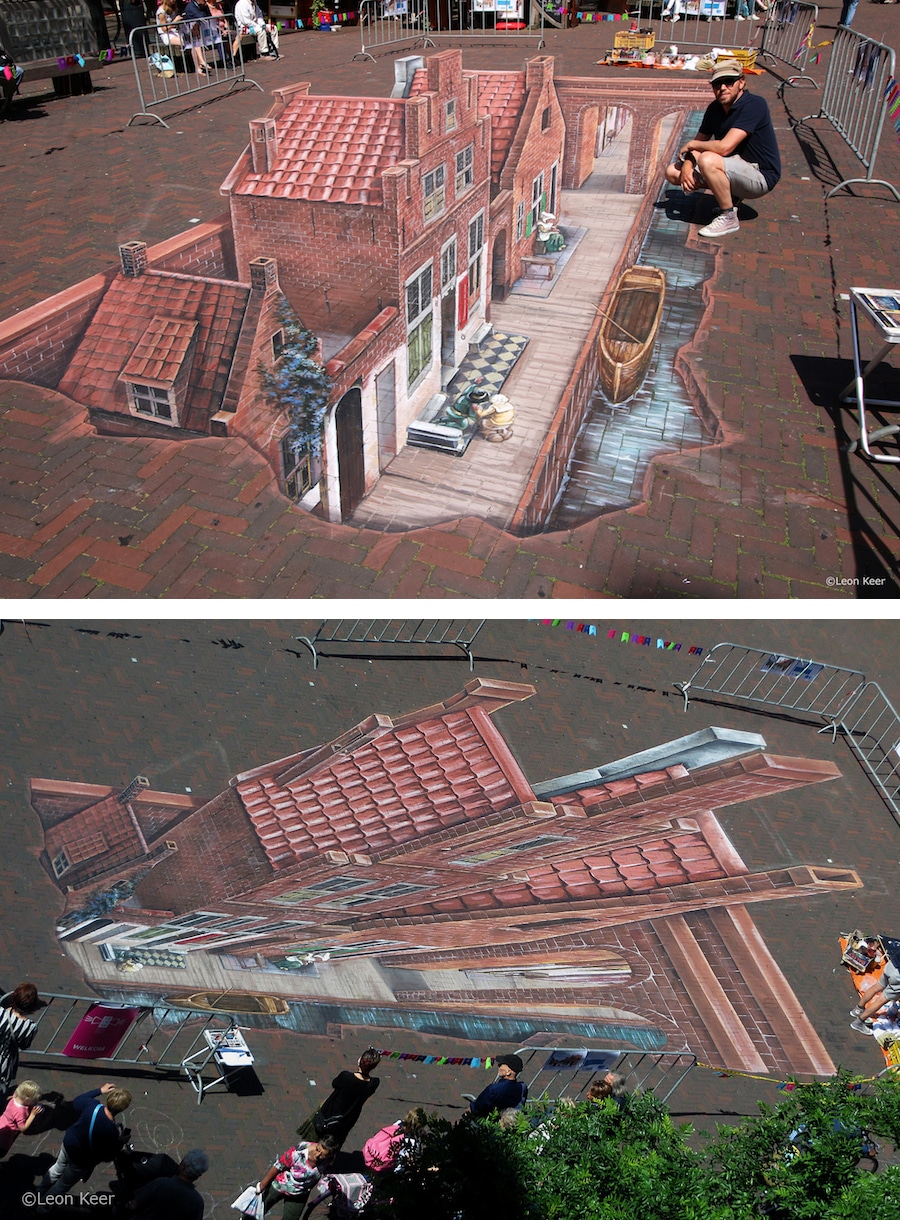
Street artists have used the power of perspective for a long time.
What we're doing is computing a homography to build a mosaic. Just like the decorative tile art of the same name, we are taking tiles of photos that we transform to overlap, and them stitching them all together into one, broader image.
Moreover, our homographies have a really funny interpretation to them. Since we are reprojecting pictures, what it geometrically looks like is that we're taking two photos which should be rotated in space (as you would spin taking the panorama), and taking a photo of the two photos. Photo-ception.

If you take a photo of two existing photos, you get one photo that unites the two together. If we can find out the right way to take the photo such that the overlap is correct, we get a panorama.
There are other ways to reproject images to make other mosaics with the own benefits and downsides, but this is what we'll use for now. Benefits with this type of mosaics? They are (relatively) easy and fast(er) to compute. Downsides? Since we are projecting onto a plane like this, we can only take panoramas up to 180° wide (can you see why?).
One Slight Issue…
While it's great that we are able to transform points with matrices, let me remind us what our goal is.
We have these two photos, where we want to transform one image's points to overlap with the other's. In terms of our matrix arithmetic from before, we have $p$ and $p'$, but no matrix $M$... Up to this point we have been finding our image points using our own matrices, but how do we find that intermediate matrix given a point and its image?
Regressions and 4-Dimensional Lines
Like homogeneous coordinates, many of you will already be familiar with solving for the intermediate matrix given a $p$ and $p'$. Let's do it with a simpler example.
If you had the points $(1,2)$ and $(6,4)$, and I needed you to find the line $y=mx+b$ that went through them, most of you would be able to do that. We'd set up a system of linear equations
and solve for $m$ and $b$ respectively. In this case, $m=\frac{2}{5}$ and $b=\frac{8}{5}$. Simple algebra with little to worry about here. What is important to note here is that we could solve for a unique $m$ and $b$, since two points define one unique line.
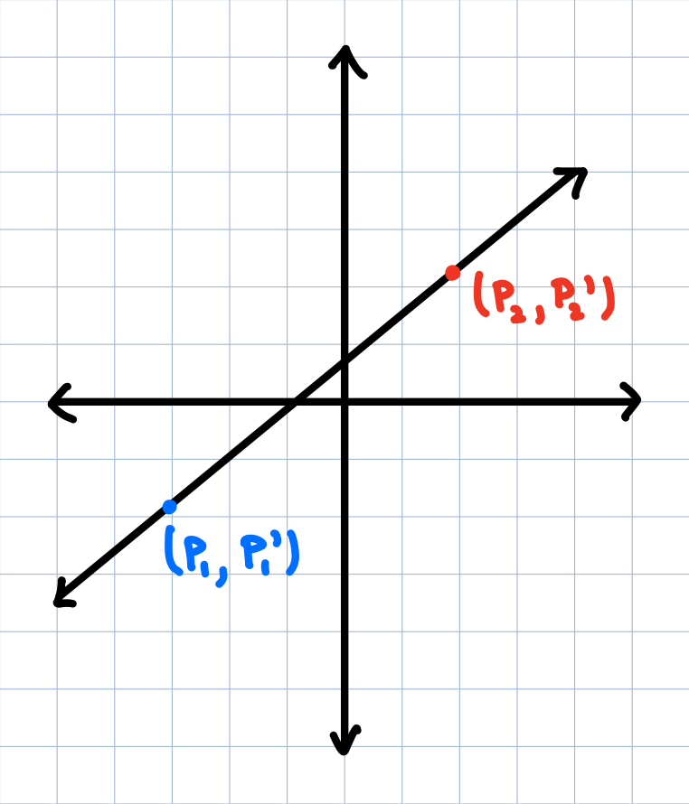
An ordinary line going between two points.
But what if I introduced a third point $(p_3,p_3')$? Or even a 4th point $(p_4,p_4')$? How do we draw a line through those 4 points? There might be a line that goes through all 4 points, but it's highly unlikely.
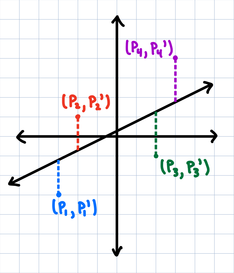
While there's no one line through all 4 points, what's the closest to a line we can get?
We may not have exact values for $m$ and $b$, but what's the best value for both to get the closest solution to this system of equations?
That's a task as simple as plugging it into a spreadsheet and doing a linear regression. More specifically, we can use the common least-squares regression where we want to minimize not the sum of the errors, but the sum of the square of the errors (as the name would suggest). For those a little more comfortable working with matrices and linear algebra, here's a more in-depth explanation of what we're doing with our data when finding a regression.
To many, this might seem like an obvious thing to do; everyone from middle schoolers to office workers have been finding trend lines forever. But what we did here is pretty useful when we think more abstractly: given a system of linear equations that correlated independent data $p$ with their dependent data $p'$, we were able to solve for the best coefficients of that system of linear equations that most closely solved the system (in the previous case was $m$ and $b$). Finding a line was a nice byproduct, but what we're really doing here is solving that system of linear equations.
Now I promise this will be helpful. Let's look at our original expanded matrix equation of $Mp = p'$.
Remember, we're working in homogeneous coordinates, so $p'$ might not land on the plane $z=1$, and we account for that with $w$ here. I also set $i=1$, since a) that corresponds with a certain scaling and is not necessarily unique vector in the land of homogeneous coordinates, and as a result, more importantly b) gives us one less variable to solve for.
Here, we will need to actually do the matrix-vector multiplication, and carrying it out nets a system of linear equations! (I know I said you won't need to know the mechanics of these operations, but it's hard to avoid it now. If you can accept this fact, that's great, but I'd recommend looking here if you are unfamiliar.)
Using the third equation in tandem with the first two…
Just like before, we can solve for $a$, $b$, $c$, $d$, $e$, $f$, $g$, and $h$ with a least-squares regression! Since we have 8 variables, at minimum we need 8 equations, or 4 pairs of $p$ and $p'$ (since each pair contains two equations: one for $x'$ and one for $y'$). Though, just like we have 10 points, generally it is better to have more data and overfit than less (we'd rather have an overall average fit, than just 4 points be exatly where we want them to be). It's weird to think of this geometrically, since what we're doing here is not finding the line between one independent variable and one dependent variable, but rather two independent variables $(x,y)$ with two corresponding dependent variables $(x',y')$; our regression exists in 4-dimensions!
Putting It All Together
Let's quickly reflect on what we've covered thus far.
- We've redefined coordinates purely with vectors, allowing us to nicely compact our image-warping transformations in matrices.
- Our original definition of coordinates failed to include translations—a key transformation. We described 2-dimensional points in 3-dimensions with homogeneous coordinates, resolving our worries.
- We then ran into ANOTHER problem in that while we knew how to warp images given the transformation matrix, we really wanted to be able to find the matrix given a starting point and an end point to map to.
- Using a least-squares regression, we were able to turn our unknown matrix equation into a system of linear equations that were much easier to work with to compute our homography (sort of, see the aside below).
Let's use this first photo to give our list of points $p$.
And we'll try to match those red points to these blue points on the second photo: our list of $p'$.
Having the computer compute the transformation matrix, we take that matrix and multiply every pixel (remember, treating them as coordinates/vectors), and warping the first image. Then, we can overlay them to see how close our points line up! If our points were well selected, and our computed homography—with the least-squares regression—has minimal error, we should get a pretty decent attempt at a panorama.
Sure, the blending isn't great, and it didn't completely fix the overlap issue, but the seams and photo stitching definitely is much nicer! And honestly, it's pretty cool seeing how the image was transformed and finding the outline of the images cross like that.
With some simple masking and basic filtering (basically averaging every pixel's color with the pixels around it), suddenly it really begins to look clean.
While this is cool, it does reveal another unfortunate downside of our choice of mosaic: if we want a uniform picture, we have to sacrifice a lot of data.
Even so, it doesn't even look that bad. All in all, though, not a bad first attempt at building a panorama.
What Next?
While we have a working prototype, we can do signficantly better. For one, I used only 10 labelled points to compute our homography, but if you use even more, it's not hard to get a better, and closer fit. With algorithms like LoFTR, finding lots of corresponding labelled points between multiple images is quick and easy.
Some really smart people made an algorithm specifically to finding high quality object matching between multiple photos. Credit: LoFTR Team
Also, since we are manually constructing our panorama, we can stitch and blend photos that have no right being together in a panorama.

Going from a well-lit to a dark photo makes for some artsy renditions (even more if you blend it a little nicer).
In a similar manner, we only conjoined two photos together, but we can easily extend this to as many photos as we want (but I can't say how well the photos towards the end will necessarily stretch).
We never really touched on our homographies, either. When we decided 10 initial points $p$ and 10 warped points $p'$, our $p'$ was decided as a result of lining up 2 photos. What if we didn't want to line up multiple photos, but rather just creatively warp a single photo?
Something not quite lined up? A simple homography can fix that for us.
This is know as rectification, as it is a means to correct for mistakes we might have had in our photo.
Finally, the last improvement we can make to our mosaics is trying new projections and warpings. If we want something even as simple as just wider, up to 360°, full views, we'll need to find something more robust than our previous approach. Or what if we wanted to make something akin to a full photosphere like from before?
What we did today was simply planar projection, or just reprojection onto a plane. We did that with homogenous coordinates. For wider, more complete mosaics, we'll need either cylindrical or spherical projection, which is exactly what it sounds like. These have their own benefits like wider field of view, but because of the nature of projecting onto a curved surface, the images being stitched together do tend to, well, curve. The type of mosaic one uses comes down to preference and artistic need.
And lastly, there are many optimizations and polishing details we could add to make our panoramas cleaner, and run faster. For instance, we never mentioned the discontinuities that could be present in warping our images with matrix multiplication. While linear transformations keep lines before the warp as lines afterwards as well, that's only helpful if our line is continuous. Pictures are not continuous! They are discrete points! So, forward warping with our matrix multiplication and finding where pixels lands can sometimes create (albeit, usually imperceptible) holes in our images, but they are there nonetheless. Instead, we can reverse warp by applying the inverse of our transformation matrix, and find what coordinates land on our original image! Not to mention different blending and masking techniques, or even just algorithmic improvements to make the code run faster. Check out the Python notebook below for more details.
For more like this and additional resources, I recommend reading these slides from UC Berkeley's introductory computer vision and computational photography class.
I hope this gave an interesting peak at the intersection of linear algebra and photography, and more over, I hope this gave you an appreciation for the math your phone goes through every time you take a panorama.
If you're interested, here's a link to a Python notebook where you can see some of my experiments during my struggle and exploration with panoramas and homographies.
Aside: Least-Squares with Linear Algebra
Okay, this previous section is really hard to describe without already knowing a fair amount of linear algebra, and it felt a little flat without having a more methodical procedure of solving a least-squares regression. I wasn't planning on including this section, but it felt incomplete otherwise. For those interested, feel free to peer over it, but this is not necessary within the scope of this post; all you need to understand is what our regression is accomplishing, thinking of that "line of best fit" idea giving rise to optimal coefficients in a overfitted system of linear equations.
Let's go back to when we were trying to find a line between two points. If you have 2 points, $(p_1, p_1')$ and $(p_2, p_2')$ being fit to the line $y=mx+b$, we have a system of linear equations like before.
We can solve this just like we did before to find $m$ and $b$, but there's another, sly way we can approach this. If we look carefully at the structure of these equations, there's actually a secret matrix relationship embedded into this system.
In a sense, that's what a matrix is: a system of linear equations, and you can freely go between either a system of linear equations or a matrix via matrix multiplication. (I know I said you won't need to know the mechanics of these operations, but it's hard to avoid it now. If you can accept this fact, that's great, but I'd recommend looking here for more details.)
If we write this in general terms, we are basically solving the equation
where $A$ is a matrix, and $b$ and $x$ are vectors, and we are solving for the latter. It might seem pointless to rewrite it, but what we're actually solving is
Since $Ax$ is exactly equal to $b$ in the 2-point case, we can solve this matrix equation fairly directly; when there's a unique, perfect solution $Ax$ is the same vector as to $b$. We were able to find a unique line with $m$ and $b$ through them, no? Just as we were able to solve the system of linear equations before, we can easily solve this with matrix inverses:
Now, let's add more points.
Now we turn this into a matrix equation like before.
We know that there's a good chance our four points don't all lie on the same line. So it's unlikely that $Ax - b = 0$. Moreover, now that our matrix $A$ isn't square, we can't just use inverses to solve for $x$. So instead, we want to get a line that gets as close to 0 (a.k.a. being a perfect fit). So our goal is to
Here, the $||x||_2$ means we're looking at the Euclidean distance (a.k.a. straight line distance) as our error for our line of best fit, and we're squaring it to get a tighter fit since small errors are kept relatively small, while large errors are weighed heavier. We know $A$ and $b$ with $x$ as our unknown—this sort of looks like a parabola-y equation! When we minimize a single variable function, we do so with the derivative. We can do the same thing here except with the multivariable equivalent: the gradient. So, we know the minimum occurs where the gradient of this function is 0.
Even if you're not familiar with multivariable calculus, much of the following should still look vaguely familiar to the chain and power rules of single-variable calculus.
All finally simplifying to the very nice formula of
I like this approach for it's intuitive roots in the geometry of single-variable calculus, but if you want a more strictly linear algebra approach, here's this excerpt from Georgia Tech that explains another proof for the same formula:
Theorem. Let $A$ be a $m \times n$ matrix and let $b$ be a vector in $\mathbb{R}^m$. The following are equivalent:
- $Ax=b$ has a unique least-squares solution.
- The columns of $A$ are linearly independent.
- $A^TA$ is invertible.
In this case, the least-squares solution is
Proof. The set of least-squares solutions of $Ax = b$ is the solution set of the consistent equation $A^TAx = A^Tb$, which is a translate of the solution set of the homogeneous equation $A^TAx = 0$. Since $A^TAx$ is a square matrix, the equivalence of [facts] 1 and 3 follows from the invertible matrix theorem. The set of least squares-solutions is also the solution set of the consistent equation $Ax=b_{\textrm{Col}(A)}$, which has a unique solution if and only if the columns of A are linearly independent.
Basically, it says if our system of linear equations contain only unique equations (i.e. no one equation is a multiple of another), we can turn our non-square matrix $A$ into a square one by multiplying by its transpose $A^T$, and solve our least squares the way we'd solve it before with inverses. In other words, if our matrix follows the criteria listed above, our minimizing solution comes from creating an equivalent equation with an invertible matrix:
Netting precisely the same formula as before.
Now, let's recall the our matrix equation from before of the homography we wanted to solve.
Then, we expanded this into 3 linear equations, and further simplified them to the following two:
This, can be rewritten as another, secret matrix equation:
Wait, we turned our original matrix equation into another one? As awful as that may look, this is much more useful than our original equation since now, all of our unknowns are in a vector instead of a matrix; it really is no different than our previous least-squares examples, and we're still solving for the vector $x$ in
So, we can still solve it like before finding
And with that, we now have also gone through what our program is doing under the hood, and have gone through some of the tedium of justifying what a least-squares regression is from a linear algebra perspective.