You're a business tycoon. You have ideas in mind but no products on hand. You need to make a quick buck now and all you have is some needlework on your belt to carry you. If you wanted to maximize profit between making hats and shirts, what combination of the two should you make? Well, let's look at what our goal is. If I make \$15 per shirt, and \$10 per hat, we can have a simple goal of
Obviously, we can't just make infinite of each wearable. We have some constraints between available cloth, printing, and effort. If you have 20 sheets of cloth, and each shirt requires $\frac{1}{2}$ of one and the hats only require $\frac{1}{5}$ of one. For printing, maybe you only have enough ink for 100 prints total. Finally, hats are hard to make, so you cap yourself at only making 70 and no more. We have a list of constraints which can be nicely added as a set of inequalities:
This isn't an easy system to solve as, well, we're not solving anything in the traditional sense by plugging in equations to one another, nor is it a standard maximization problem where we can take some form of a gradient since every equation here is a line, so we would only get constants that give us no new information.
This type of problem where we want to maximize a linear equation that is also bound by a set of linear restraints is called a linear program. These types of problems are called specifically programs as you'll see that we have analytic ways to find solutions, but to find the best solution requires some well-crafted algorithms to make solving them faster and more efficient. Before we can understand the 2, and later the general $n$, variable set up, let's try an easier case.
1D Linear Program
As with all problems, let's try and cut back on degrees of freedom so we can really focus on what's going on here. Instead of maximizing a function of 2 variables, let's do a function of 1 variable.
This isn't all that interesting, as I'm sure the answer is popping out almost immediately: $\max(3x)=30$ from since we can only have at most 10 of variable $x$ from the first constraint. What will become an important concept later is how we visualize these solutions to linear programs, so let's graph our inequalities on a number line to represent the quantity of variable $x$.
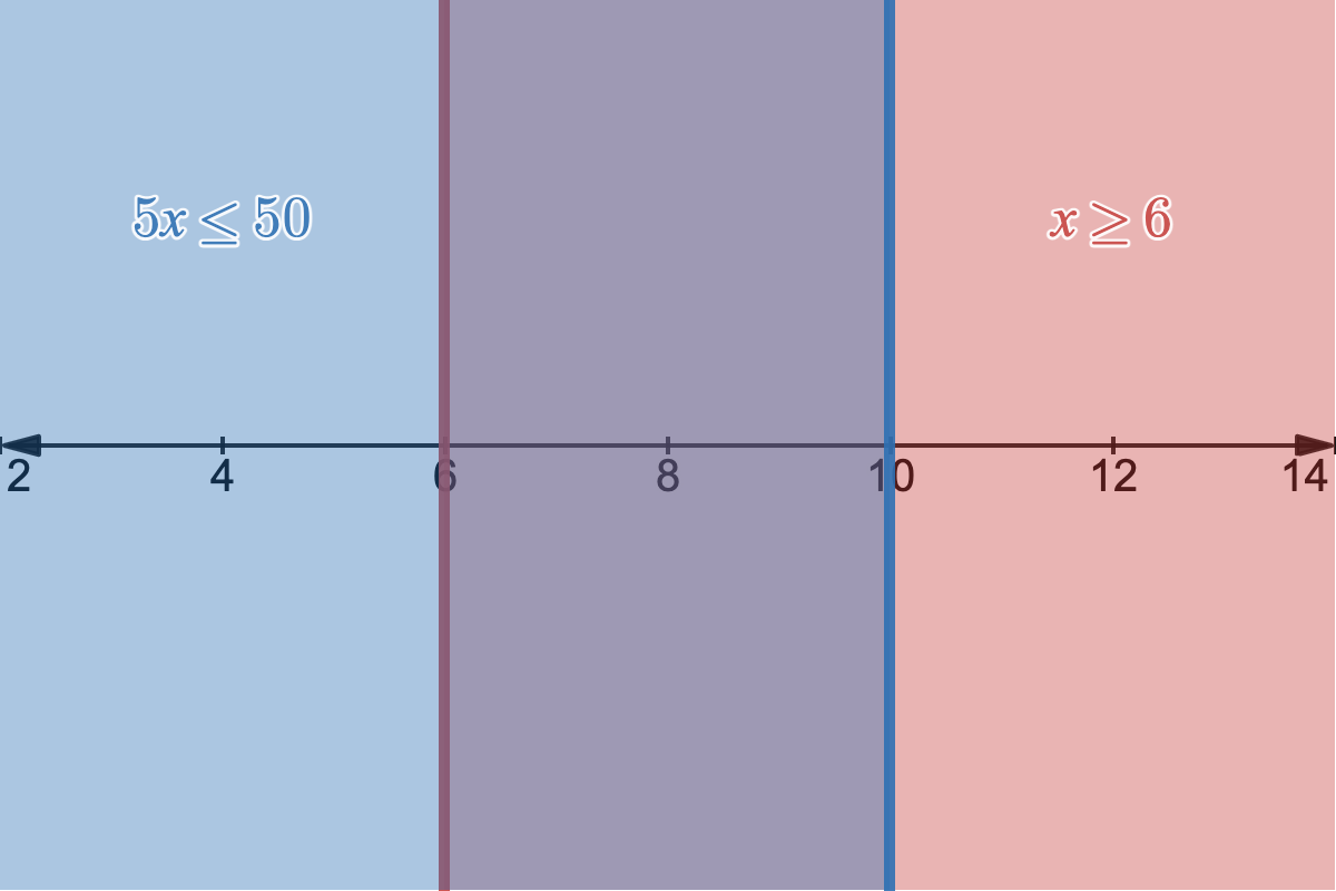
Feasiblity region graphed for our 1-variable linear program.
In blue, we have our first constraint of showing all values of $x$ that satisfy $5x \leq 50$, and in red we have our second constraint showing all $x$ that satisfy $x \geq 6$. Where those two regions overlap in the purple-ish area is the feasibility region, as well, it's the area where all of our constraints are satisfied and where feasible values of $x$ lie. The feasibility region defines a polytope, a generalization of the 2D polygon and 3D polyhedron. The key takeaway is that our solution of $x=10$ is an edge case: it lies on the furthest possible boundary of our feasibility region.
This makes sense for two reasons. 1) We want to always be looking to maximize or minimize our objective function ($3x$, in this case) so if we can add more or less of $x$ to our solution, we want to do that depending on our goal. This is a more intuitive way to show reason 2) our function is linear, so as long as we go in one direction, it will always be increasing or decreasing. Let's add the $y$-axis into this graph and let $y=3x$ to see the value of the function we're maximizing at different values of $x$.
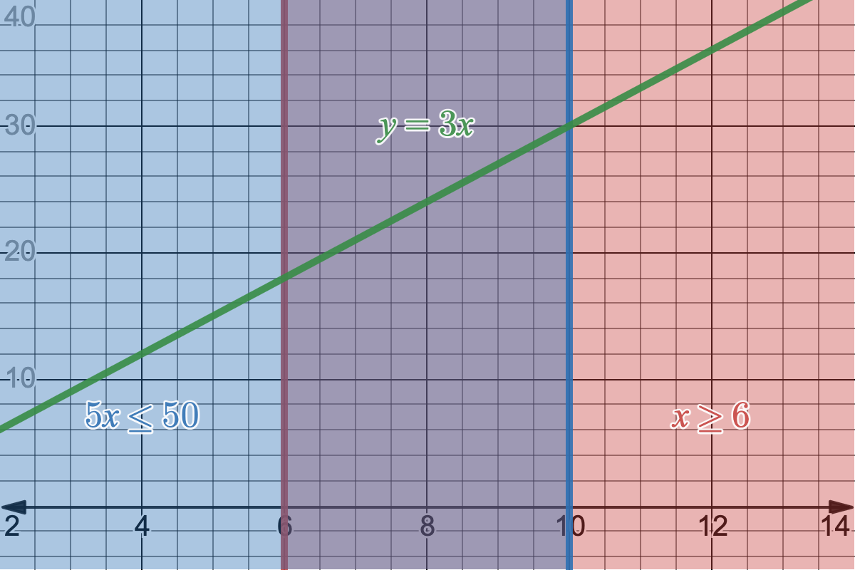
Objective function $y=3x$ plotted with an extra dimension.
Since our objective function is linear, it is directly proportional to $x$, so as $x$ increases or decreases, $y$ also has to only increase or decrease with no chance of weird curves or bends in its function. So if we want to maximize our function, we just want to walk in the direction of $x$ that does so until we hit the edge of our feasiblity region. Similarly, if we wanted to minimize it, we'd walk the other way along $x$ that decreases $y$.
With this in mind, we can now go back to our original 2 variable case.
2D Linear Program
Recalling what our original setup was
Let's plot our feasibility region like we did before. Only now, it'll be a 2-dimensional region instead of just the number line. We'll put $s$ for shirts on the $x$-axis and $h$ for hats on the $y$-axis.

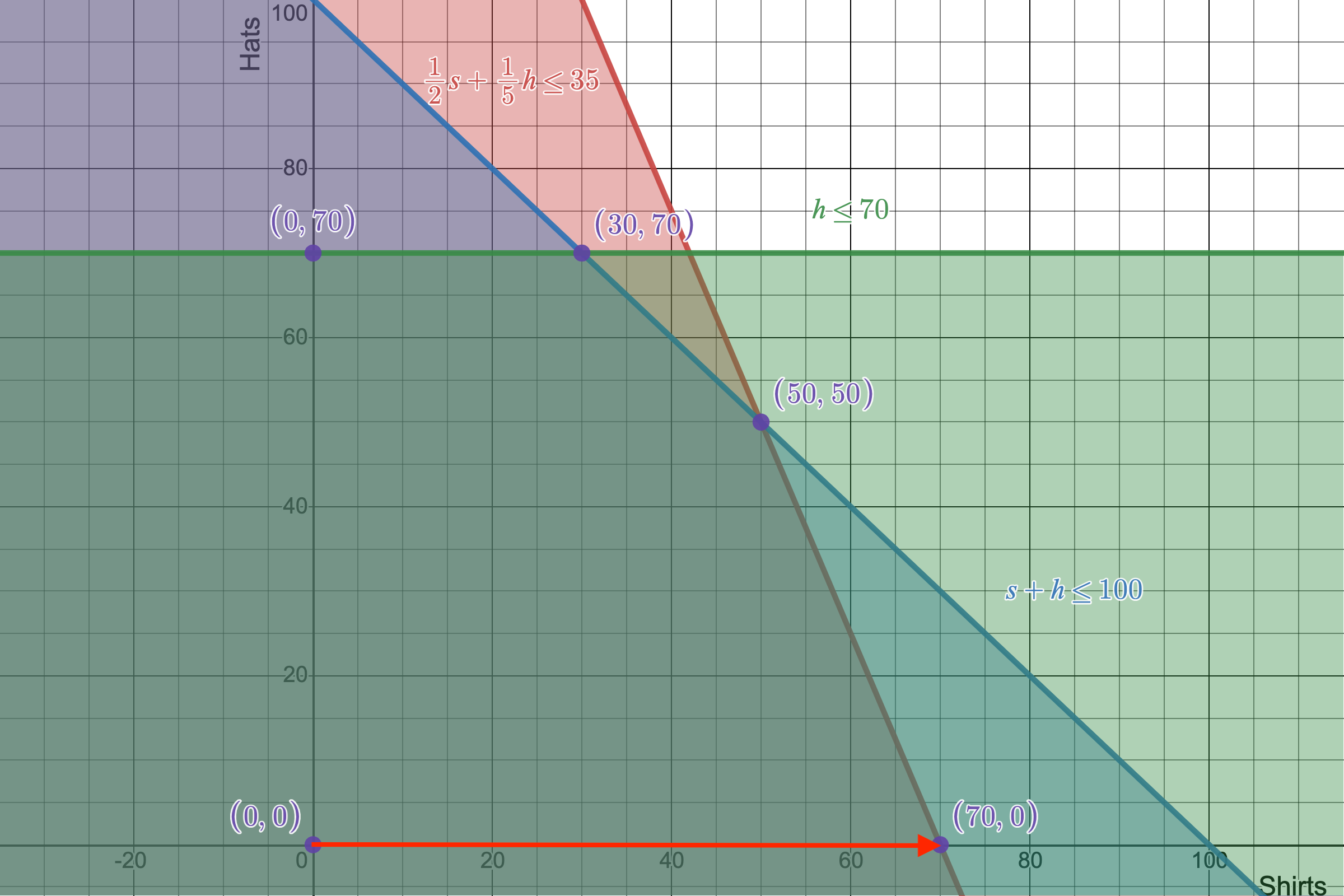
5 vertices map out our 2D linear program's feasibile region, meaning there are 5 possible points that can be our optimal solution.
Just as in the 1-variable case, our solution for maximizing our objective function should lie at the edge of our feasible region. I've marked the feasible region's defining vertices in purple. It's worth pointing out that I have added an additional vertex not defined by our original constraints, and that's the vertex $(0,0)$. This is aptly called the non-negativity constraints as it, well, constrains our variables to be non-negative (shocking, right). These tend to be a requirement for some minimization cases just so that we don't end up with problem of running into a pair of negaively infinite numbers as our solution, which obviously doesn't make sense.
Although what I said about our solution being on the edge of the region isn't true, I can tell you more about our maximum solution: it will (usually) be one of the vertices of our feasible region. If you want a more math-based explanation, check this out, but there's a very intuitive way to view think of this, especially with a 2-variable linear program.
Remember how in the 1D case, our objective function $y=3x$ could be represent as a line? We can do a similar idea and add a third $z$-axis to our 2D problem and get $z=15s+10h$. This equation gives us a 3-dimensional plane as we encode the number of shirts, hats, and the amount of money they profit. Our constraints are also planes, acting as curtain-like walls extending forever vertically in the $z$-axis (as all values of $z$ will satisfy whatever values of $s$ and $h$ that lie on the line). Now, imagine our objective function plane of $z=15s+10h$ to be like a tilted table, and we place a ball on it to roll, what does the ball do? Well, the ball will just roll down the incline to the lowest point gravity will push it down. Normally, the ball will roll down forever and ever as our table extends infinitely in all directions, but we have our constraining walls to stop the ball. As soon as the ball hits a wall, it'll continue to slide down that wall as long as the ground tilts downward. It'll only stop if another wall pushes it into a corner, which is where our constraints form a vertex. Isn't that neat? The only times this won't be true is if one of our constraints form a wall that is exactly perpendicular to the direction the ball is rolling, in which case you will have a line segment worth of solutions (which includes two vertices at the end of it). This specific logic applies to finding minimums of our objective function, but you can also think of the reverse for maximums with a tilted ceiling and a balloon instead of a ball. It's basically a streamlined version of gradient descent since the gradient of the plane is always constant.
So if you manually check all 5 vertices, you'll find that a combination of $(50 \textrm{ shirts}, 50 \textrm{ hats})$ gives the optimal combination of $1250 profit. Not bad.
The Simplex Algorithm
Not to dismiss the wonders of guess-and-check, but it only worked well for us due to the small number of variables and constraints we had. As we tackle more complex and intricate problems, we want to be able to solve linear programs much quicker and more efficiently. There are many algorithms that have been developed for LP optimization with varying motives, but the first one was George Dantzig's simplex algorithm.
The simplex algorithm is essentially a systematic way for us to narrow our guess-and-check quickly. We start at some vertex, and then travel edges of the feasbile region between vertices until it lands on the optimal solution. The idea is by turning our constraints into a matrix, we can use Gaussian elimination to move between possible candidate solutions until no improvement to our objective function can be made. Let's use our original 2-variable problem to try it out.
To start, we're going to turn these inequalities into equations by adding slack variables. To avoid confusing variable names later, I have replaced $s$ with $x$ and $h$ with $y$. The idea is that if our inequalities are anything less than the right-hand side, we should be able to cover that excess by adding an extra variable to make it equal. Rewriting all of our inequalities (including the objective function with a new objective variable $z$) into equations, we get
This is a system of linear equations we can encode as an augmented matrix!
Here are some things to identify in our simplex tableau above. The first row is more a convenience than anything, keeping track of which column corresponds to each variable. The second, third, and fourth rows all correspond to some constraint we have rewritten as equations with slack. The fifth and final row is our objective function which we are trying to maximize. So, by default, we assume we start at the point $(0,0)$ in our feasibility region. Yes, it is a vertex and therefore a candidate solution, but obviously it's not the maximum solution we want, giving us a whopping $z=0$. How do we find the next candidate point? Well we first want to identify which of our variables would increase $z$ the quickest. Well, notice that $x$ has a coefficient of $-15$ in the objective function final row, while $y$ has only a value of $-10$ (we call these numbers indicators). This means for every unit of $x$, we gain an additional \$15 contrasting an additional \$10 from a singular unit of $y$. Since $x$ increases $z$ faster than $y$ does, let's focus on column 1.
If we're going to increase $x$ to increase $z$, how do we know how much to increase it by? We can use our handy constraints to tell us exactly that. What we do is we take each value in the $x$ column and divide its associated row's constraint by that value. So, for the $x$ variable we have
Now why is this helpful? These divisions tell us the maximum amount of $x$ we can have according to each constraint (as we assume $y$ can be 0). So, if $\frac{1}{2}x + \frac{1}{5}y \leq 35$, then $x$ can be at most 70 without breaking that constraint. Similarly, $x$ can be at most 100 for the second constraint, and there's no limit for $x$ on the third constraint since it doesn't impact that inequality. So, this tells us we should use the first row as our guiding row! This is because if we used the second row with a maximum of 100, we would be violating our first constraint that $x \leq 70$. So, we call $\frac{1}{2}$ our pivot as we use that value to shift our focus from one vertex solution to another. We use our pivot to do Gaussian elimination, and create 0s in that column's other rows to land us at a new vertex.
$\downarrow$
$R_2 - 2R_1$
$R_3 - 0R_1$
$R_4 + 30R_1$
$\downarrow$
$ \begin{array}{cccccc|c} {\bf x} & {\bf y} & {\bf s_1} & {\bf s_2} & {\bf s_3} & {\bf z} & \textbf{constraints} \\ \hline \frac{1}{2} & \frac{1}{5} & 1 & 0 & 0 & 0 & 35 \\ 0 & \frac{3}{5} & -2 & 1 & 0 & 0 & 30 \\ 0 & 1 & 0 & 0 & 1 & 0 & 70 \\ \hline 0 & -4 & 30 & 0 & 0 & 1 & 1050 \\ \end{array} $
This new vertex we have arrived at is exactly the solution you get only focusing on achieving a maximum $x$ at the point $(70,0)$, which is in fact, the solution with the most units of $x$.
The first step in our simplex algorithm visualized as we walk the edge between $(0,0)$ to $(70,0)$. This first step is definitely a better solution than before, but how can we tell if it is the best one?
\$1050 is definitely much better than netting \$0, but how do we know if we can make more? Going back to our objective function in the last row of our tableau, there's a $-4$ in the $y$ column, and as before, should mean there's a potential to increase profit by adding some $y$ component to our solution. Before we do that though, notice how some of our constraints have changed. $R_2$ used to denote $x+y+s_2=100$, but now it shows $\frac{3}{5}y - 2s_1 + s_2 = 30$, or as an inequality, $\frac{3}{5}y \leq 30$. What caused our constraint to change? It has to do with the fact we added rows together. Let's analyze the two original constraints in question of $R_1$ and $R_2$.
We can then treat these as a system of equations like we did with Guassian elimination, and perform the same operation as we did before with $R_2 - 2R_1$.
The important part to notice is that we're subtracting from the blue region $\color{blue}{R_2}$ and expecting a positive result (since both $x$ and $y$ must be greater than 0). This can only happen for our feasible region where the blue area $\color{blue}{R_2}$ is strictly greater than the red area $\color{red}{R_1}$. This appears only when $\color{red}{R_1}$ is contained within $\color{blue}{R_2}$. The $y$-value we solved for of $\frac{3}{5}y \leq 30$ is that maximum $y$ value of which that holds true. Anything above $(50,50)$ and suddenly the blue region is contained by the red, but anything below is fair game.
Our constraints haven't actually changed, they actually narrowed in given new information of which boundaries we are at with our current candidate solutions.
With that justified, we can now move on to repeating our pivoting process like before. In our new tableau, the $y$ column has a value of $-4$ in the indicators, meaning we have a possibility to increase $z$ by changing increasing $y$. Going through our process all over again to find and use the pivot:
With a new pivot found...
$\downarrow$
$3R_1 - R_2$
$3R_3 - 5R_2$
$3R_4 + 20R_2$
$\downarrow$
$ \begin{array}{cccccc|c} {\bf x} & {\bf y} & {\bf s_1} & {\bf s_2} & {\bf s_3} & {\bf z} & \textbf{constraints} \\ \hline \frac{3}{2} & 0 & 5 & -1 & 0 & 0 & 75 \\ 0 & \frac{3}{5} & -2 & 1 & 0 & 0 & 30 \\ 0 & 0 & 10 & -5 & 3 & 0 & 60 \\ \hline 0 & 0 & 50 & 20 & 0 & 3 & 3750 \\ \end{array} $
There are no more negative numbers in the objective function row's indicators, so this should be our optimal solution! This is because of the actual equation that row represents:
$3z = 3750 - 50s_1 - 20s_2$
Since every variable, including our slack variables $s_1$ and $s_2$, is non-negative, the maximum our objective function can be is $3z=3750$ with both $s_1$ and $s_2$ equal to 0. So, while we may be done doing computing our solution, we should simplify our tableau to make it more readable. Let's make $x$, $y$, $z$, and $s_3$—our non-zero variables—have coefficients of 1 so we can easily find their values.
Our second step in the simplex algorithm brought us to our optimal solution of $x=50$, $y=50$, $s_1=0$, $s_2=0$, $s_3=20$, and $z=1250$.
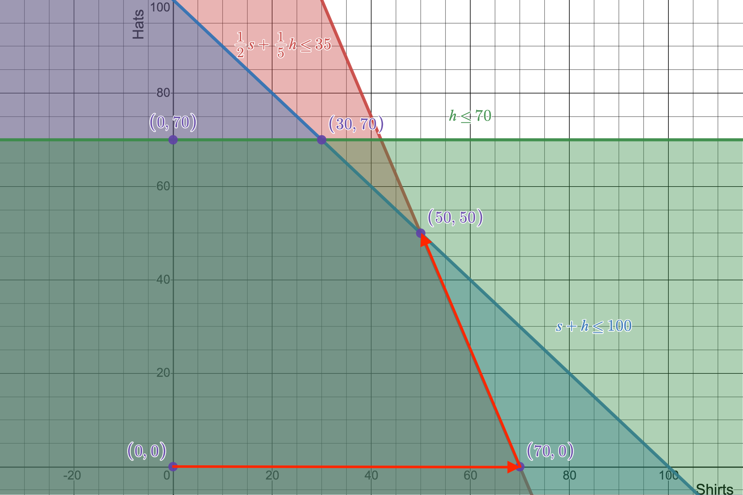
The second and final step in the simplex algorithm takes us from our last candidate solution $(70,0)$ to the optimal vertex of $(50,50)$.
Here's a summary of the simplex algorithm to solve linear programs:
- Rewrite the objective function and constraints into equations with slack variables.
- Create the initial simplex tableau using the newly written equations.
- Identify the most negative indicator to find the pivot variable.
- Calculate quotients to find upper bounds on the pivot variable, and select the smallest quotient; this is the pivot for this iteration.
- Using Gaussian elimination and row operations to turn all other values in the column to 0 using the pivot.
- If any negative indicators remain after all row operations, repeat steps 3–5.
- If no negative indicators remain, we are done and at the optimal solution$^*$!
While we only looked at 1- and 2-dimensional linear programs, remember that this can work for as many variables as you'd like, which is nice since I don't want to deal with imagining a ball rolling down a 12-dimensional tabletop to find my function minimum. There is a small asterisk though, since sometimes the simplex algorithm can "stall" or "cycle", resulting in no net improvements of the objective function. Fortunately other algorithms based on other concepts have been built to not just be quicker, but avoid degenerate cases stalling and cycling.
Sensitivity and Slack Analysis
What the values of $x$, $y$, and $z$ should be clear as those correspond to the point on the feasible region and maximum of the function, but what do the values of $s_1$, $s_2$, and $s_3$ mean? Recall that these are our slack variables as these are the variables that turned our constraining inequalities into equations by accounting for any slack in the constraints themselves. So, if we have 0 slack for one of our constraints, it means that we are using up as much of that constraint as we can; there is no slack to account for, and the corresponding slack variable is 0. If there is slack, it means we are not using up a constraint to its fullest potential. Recall our third constraint was
Also remember that our optimal solution included that $y=50$. We set a cap of $y=70$, but we are only using 50 of those possible 70 units. $s_3$ tells us that in the third constraint, we have an excess of 20 unused constraining units. In that same sense, $s_1$ and $s_2$ tell us we have 0 wasted resources for the first and second constraints. This also tells us that we are precisely at the vertex of where the first and second constraints graphically meet, since our solution is on the edge of both inequalities.
That's not the only information our slack variables tell us, though. You can also find how sensitive our result is in the final row of our tableau. The $\frac{50}{3}$ and $\frac{20}{3}$ tells us for every additional unit we add to constraints of $R_1$ or $R_2$, we will make an additional \$ $\frac{50}{3}$ or \$ $\frac{20}{3}$ respectively since $\frac{50}{3}(s_1 + 1) = \frac{50}{3}s_1 + \frac{50}{3}$. These are called shadow prices of our objective function. If you want to read more about shadow prices and other marginal analysis such as reduced costs, MIT OpenCourseWare has you covered, but for now there are a few cool extensions of linear programming I want to cover.
Duality and Dual Problems
Even though we have a systematic way to find our ideal solution to a linear program, we could have quickly found some facts about our solution before we started. Again, here is our previous, 2-variable linear program.
In our 1st constraint, we could have equivalently rewritten it as
by multiplying both sides by 60. Furthermore, since both $x$ and $y$ are greater than 0, we can also compare it to our objective function.
So we now have an upper bound on our objective function: we know for sure it has to be less than 2100. We can be even smarter about this and do a similar process with our second constraint. By multiplying both sides of the second constraint by 15, we can say
which gives us an even tighter upper bound on our optimal solution. This is the heart of duality: instead of trying to directly solve our maximization problem, we can turn it into an equivalent minimization problem to find the lowest upper bound of our objective function, indirectly solving it.
We can generalize this by multiplying all of our constraints by a scalar $a_i$ for each constraint and adding them all together.
Adding these all together, we get a unifying inequality of
Lastly, remember this is supposed to be an upper bound on our objective function, so we set this all greater than our objective function which I've highlighted in red. In our first few tries to bound the problem, we had $(a_1, a_2, a_3)$ equal $(60,0,0)$ and $(0,15,0)$ respectively. We can summarize our goal of minimizing the right-hand side while maintaining all these inequalities as true as
This looks like another linear program! We originally started with a primal problem with 2 variables and 3 constraints and used it to formulate its dual problem with 3 variables and 2 constraints!
But, what even is the purpose of this dual formulation? We already have a way to solve for an optimal solution, why needlessly copmlicate it with an extra intermediary step? The dual problem is useful as it allows us to readily access a lot of the sensitivity analysis. Each variable $a_i$ we're solving in the dual problem corresponds to the optimal shadow price (marginal utility of a resource) of the $i^\textrm{th}$ constraint in the primal problem.
Let's take a quick look back at our primal problem's solution. Recall that it had shadow prices of \$ $\frac{50}{3}$ for the first constraint of $\frac{1}{2}x + \frac{1}{5}y \leq \color{blue}{35}$, a shadow price of \$ $\frac{20}{3}$ for the second constraint of $x + y \leq \color{blue}{100}$, and a final shadow price of $0$ for the third constraint of $y \leq \color{blue}{70}$. If we value our total resources (highlighted in blue) at their marginal costs, we get that
which is precisely the optimal profit we got originally from the primal problem. The leading principle of a dual problem is that if we can solve for the optimal marginal profits of each resource, then we know implicitly how much of that item we should buy given the total selling price of each primal variable.
We try to minimize the cost of our primal constraints, while trying to ensure our dual constraints satisfy the coefficients of the primal objective function. In the case of shirt and hat selling, we want our marginal profits to at least equal the price we want to sell our products at. Even more interestingly, just like how our dual variables are equal to the primal shadow prices, the dual shadow prices are equal to the primal variables! Everything has been switched around!
Curiosities aside, we still haven't talked about many of the reasons why analyzing dual problems is useful. Here's a rundown of some of the benefits of duality:
- Sometimes it's just easier: As you just saw, we turned a problem of 2 variables and 3 constraints into one of 3 variables and 2 constraints, and turned it from a question of maximization to one of minimization. For problems with few variables and lots of constraints, it's usually much easier to turn it into a problem with lots of variables and fewer constraints as every constraint in the problem will add some number of extra vertices for algorithms like the simplex to check, making it less efficient to check every case.
- Feasibility and boundedness: Sometimes a linear program will have no solutions whatsoever to check (imagine constraints like $x \geq 0$ and $x \leq 0$; can't be both at the same time). If the primal is unbounded (think no non-negativity constraints), then the dual is infeasible, and vice versa.
- Specialized algorithms and theorems: Beyond optimizing business plans, duality has found its way into combinatorics, graph theory, and even into the fame of game theory as a means to prove the minimax theorem for zero-sum games. Many more results like these tend to stem out of the Weak and Strong Duality Theorems (Weak Duality talks about how a dual problem can set an upper bound to a primal soultion, and Strong Duality says it can find the optimal primal solution).
Duality is a powerful concept not just in linear programming, but frequently pops up in other areas of math and recognizing when you can represent one problem with another is a great tool to have in your back pocket.
Conclusion
Linear programming is only one small niche of optimization study, but the depth and applicability in its simple premises is wildly effective. Starting out in the 40s with Dantzig's original simplex algorith, it has grown to affect much of computer science and math to systematically solve otherwise impossibly long computations. Even now, variations of the original linear programming formulation is still being researched with new methods to not only solve them, but also adding new fundamental restrictions to the problem. If you were a car manufacturer that wanted to know the optimal distribution of models to produce, you can't just make 41237.7963 cars; you would only care about integer solutions, and thus integer linear programming (ILP) was born. Linear programming's innate utility in optimization has lent itself kindly to modern applications, but from ILP, to the even crazier mixed-integer linear programming with a combination of integer and non-integer variables, as well as duality, LP has found itself touching every corner of math from combinatorics to graph theory as a simple multidimensional geometric encoding of a constraint function.