Delta Thoughts

Introduction

Let me propose a question to start. Try to solve the following:

An infinite power tower which supposedly equals 2? Seems unlikely, but those familiar with these infinite-operation type problems likely know the strategy to solve this. Notice how there's a copy of our equation stacked on top of itself.

Since we know that equation in the box is equal to 2 because it's a duplicate of our original equation, we can easily reduce the problem down to something much more manageable.

So, raising $\sqrt{2}$ to itself over and over again equals 2. What other equations can we solve? Let's try this one.

Using the same strategy as before, this one is trivial.

Which is… the same answer as before? How can $f(x) = \sqrt{2}^x$ iterated over itself equal both 2 and 4 at the same time? When in doubt, we can ask our calculator for some confirmation.

Estimation with Python

With some simple Python, we can get a pretty good approximation quickly.

import math
def f(x):
    temp = x
    for i in range(1000):
        temp = math.sqrt(2)**temp
    return temp
print(f(1))

The above code creates and evaluates a power tower 1000 numbers tall, giving us an approximation of 2.0000000000000004, which is pretty close to 2. So, is 4 anywhere to be seen? Actually, yeah; our solution wasn't completely false. Notice that at the end of the script it says f(1). That 1 is our seed value. Since our power tower can't be infinite in order to get a calculable approximation, we need to cut it off after some amount (in this case, 1000 numbers high). In order to do that, though, there has to be some number there at the top of that power tower. In this case it was 1, but it can be anything as we constantly plug our output back into our input, in the case of an infinitely stacked power tower, that seed value is negligible. Let's see what happens if that is changed to f(4).

print(f(4))

Due to rounding, our script actually blows up to infinity with f(4), but we can reason this out by hand. If we start with 4, then our first output of iteration will be $\sqrt{2}^4 = 4$. Since 4 is our output, that's our new input. But since 4 was also our seed value, it'll just constantly output 4 at every iteration. So 4 is a convergent value (as we can only calculate finite approximations) to the infinite power tower of $\sqrt{2}$, but only for its seed value. To better understand this, we can use a tool known as a cobweb plot.

Cobwebs

Cobweb plots are a simple, elegant method to model iterative functions in the Cartesian plane by utilizing a seemingly mundane auxiliary function: $y = x$. What is probably the first graphs people are taught in elementary school is one of the most helpful in modeling these complicated and otherwise impossible to view functions. Here's how to make a cobweb plot: 1) Plot the function to be iterated on (in this case, $f(x) = \sqrt{2}^x$) and $y = x$ together. 2) Pick a seed value to start iterating on. 3) Alternately draw vertical and horizontal lines within bounds of each graph for as many iterations as one needs. Steps 1 and 2 should be clear enough as they're fairly similar to what we did above, but Step 3 might need a visual to go along with it.

Here's the first step's resulting plot:

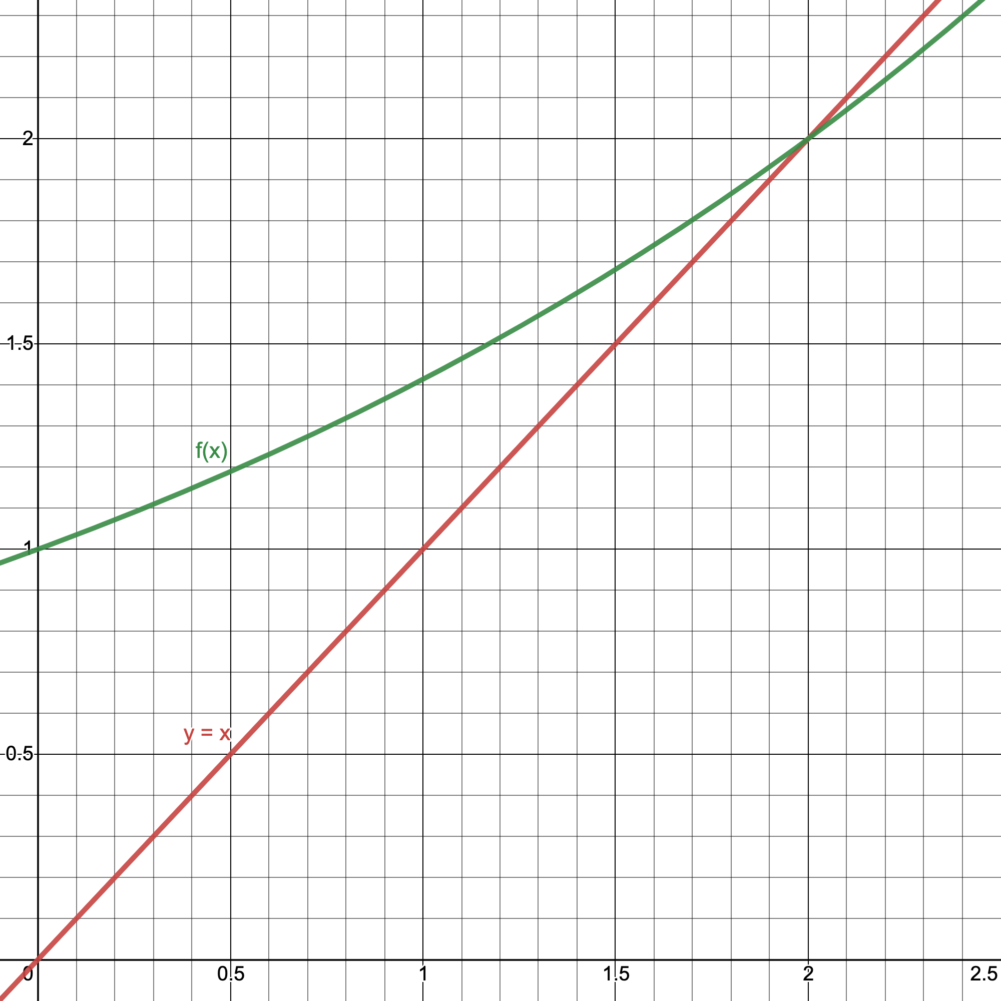
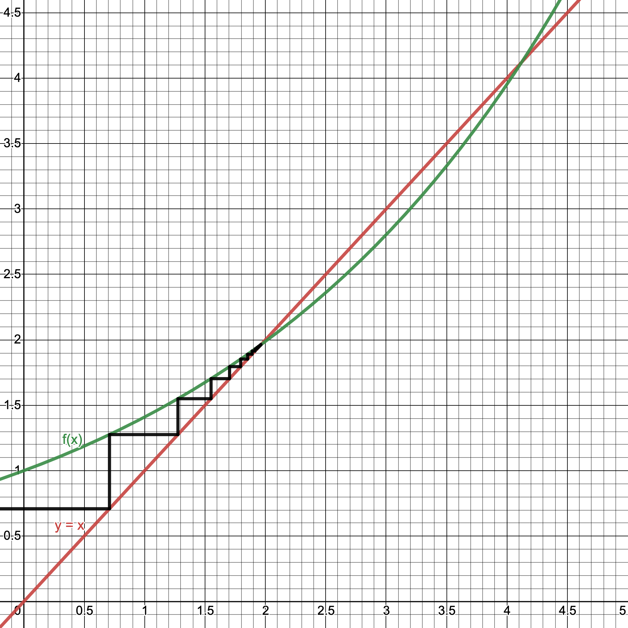
Nothing too crazy. The green graph is our $f(x) = \sqrt{2}^x$, while the red graph is our $y = x$. For Step 2 we'll pick $x = 1$ as our seed value as we did before. This is where the magic of Step 3 comes in: from $x = 1$, we'll draw a vertical line from the red graph until it intersects at the green graph.

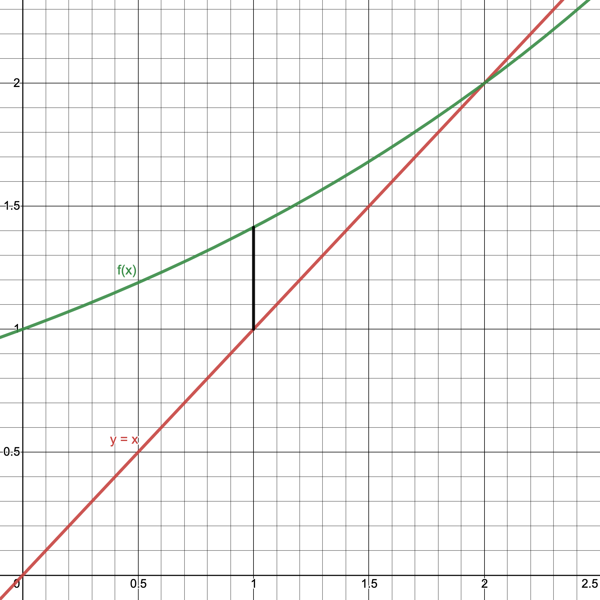
Now we have a line segment with points $(1,1)\rightarrow(1,f(1))$. This step is equivalent to plugging in 1 into the top of our power tower, geometrically doing the operation of $f(x)$. Since we just a drew a vertical line, we now draw a horizontal one from the green graph $f(x)$ until it intersects the red one $y = x$.

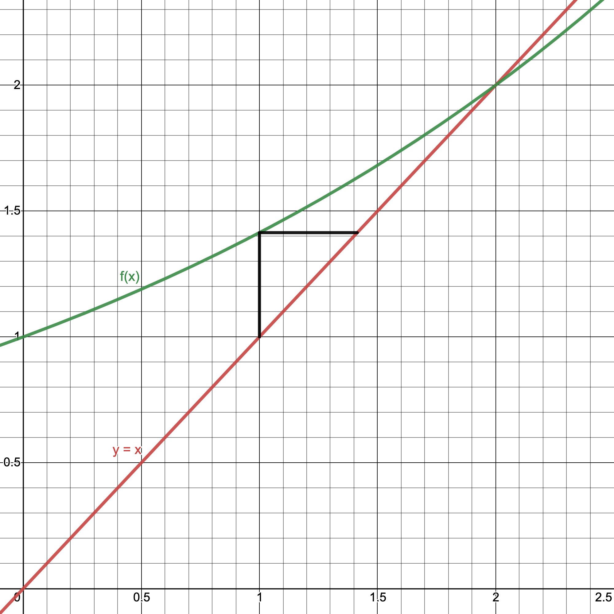
Now we have a new line segment from $(1,f(1))\rightarrow(f(1),f(1))$. You can probably see where this is going. Now that we have a new point at $x = f(1)$, we can draw a new vertical line until it hits the green graph, geometrically finding the value of $f(f(1))$, performing our repeated operation! We can do this series of horizontal to vertical lines as many times as we want to get as many iterations of our repeated function as we want!

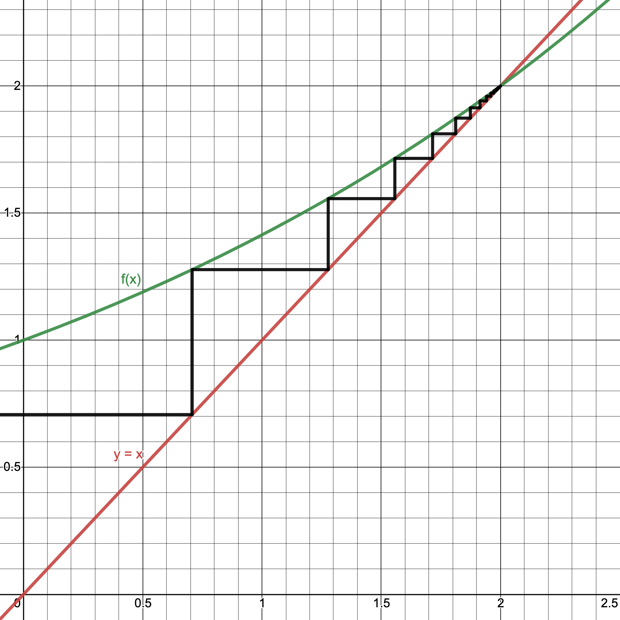
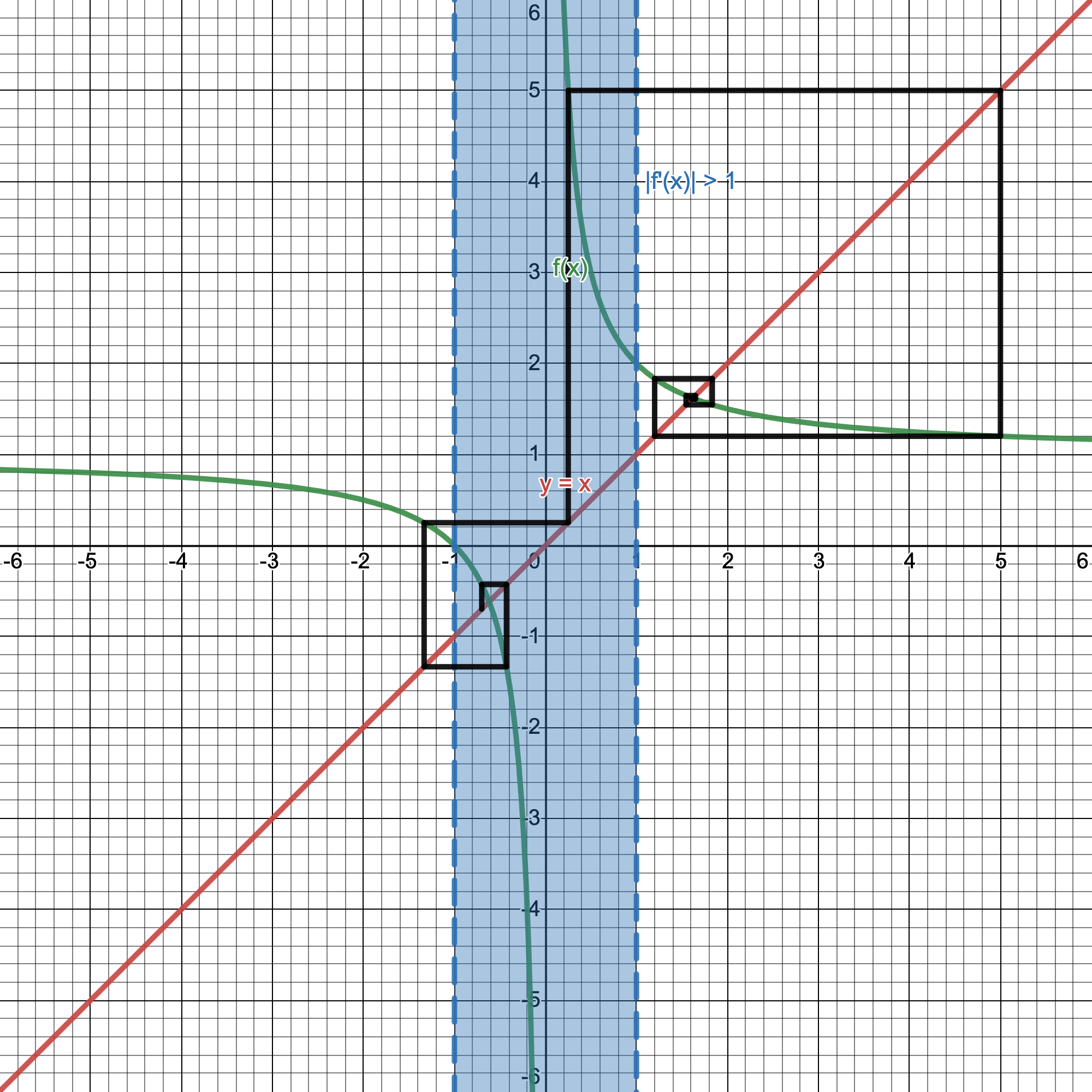
Now you can probably see why this is called a cobweb plot, as we weave back and forth creating a net-like shape between the graphs (and it only gets more wild looking with different iterative functions!). Even in the previous graph where I set the seed value to be $x=-1$, our graph still quickly hones in on evaluating to $x = 2$ for the $\sqrt{2}$ power tower, just where it happens to be the intersection of our two plots. This is a pretty narrow scope of our graph, though; let's zoom out and see more of this plot.

There's also an intersection at $x=4$! Even with all of this, I don't think it would be wrong to feel that $x=4$ should not be a solution to some extent. Even though, it clearly shows a lot of the same characteristics that $x=2$ does, it still feels weird for this to be considered an answer, or at least to the same extent that $x=2$ is. For any seed $x<4$, our iteration converges to $x=2$, and for any $x>4$, it diverges. Only at $x=4$ does our repeated power tower equal 4. To properly understand this, we'll need to utilize derivatives.

Derivatives and Sensitivity

The classic definition of the derivative $f'(x)$ is a function that returns the slope of $f(x)$ at every point $x$. While this definition of the derivative isn't wrong, it is fairly limiting when only considered in the contexts of slopes. We can reframe the idea of a derivative not to be the slope of a function at a point $(a,f(a))$ but rather how sensitive the function is at the point $(a,f(a))$. This will be more apparent if we plot our $f(x)=\sqrt{2}^x$ in a new way.

You can generate the above plot with the following Python:

import numpy as np
import matplotlib.pyplot as plt

def f(x):
  return np.sqrt(2)**x
inp = np.linspace(-5,5,40)
out = [f(n) for n in inp]
d = 10
fig = plt.figure(figsize=(20,4))
axes = plt.gca()
axes.set_xlim([-5.3,5.3])
axes.set_ylim([-6,6])
plt.scatter(inp, [d/2 for n in range(len(inp))])
plt.scatter(out, [-d/2 for n in range(len(out))])
for n in range(len(inp)):
  plt.plot([inp[n], out[n]], [d/2, -d/2], color='green')

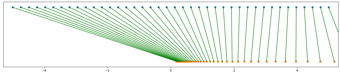
This basically just took the $y$-axis of our Cartesian graph and rotated it $90^\circ$. The blue dots represent the preimage of points $x$, while the orange dots represent their associated transformations under $f(x)$ with green lines connecting them. Just looking at it, it's consistent with our Cartesian graph as $f(x)$ never goes below 0, which makes sense as an exponential is always positive. The reason why we want this graph as it guides the intuition behind this idea of sensitivity and the derivative.

Notice the dots around $x=-3$ in the preimage (blue) points. They all get mapped and squished down near $.354$ under $f(x)$; they get tightly pressed together. But just how tightly pressed together are they? That's exactly what the derivative tells us! For a small change $dx$, we want to know how much that changes the output $df$. In this case, $f(x)=\sqrt{2}^x \rightarrow f'(x)=\sqrt{2}^x\cdot\ln{\sqrt{2}}$. Plugging in $f'(-3)=.1225$. This means that around $x=-3$, the ratio between how much the points around it changes under $f(x)$ is $.1225$, in other words, the area around $x=-3$ appears to have shrunk inward by a factor of $.1225$. In the contexts of slopes, this ratio would be the slope of our tangent line, telling us how tall $df$ would be relative to $dx$. Since the derivative $f(-3)$ is small, we can say that $f(x)$ is not very sensitive around $x=-3$, as a small change in input from $-3$ will still evaluate to about the same value.

Now let's look on the right half of the graph. Trying $f'(4.5)=1.6486$ would imply under our previous logic, that we'd expect points to stretch away from $x=4.5$ by a factor of $1.6486$. Just by looking at our plot, that's not so hard to believe. This means that our $f(x)$ is sort of sensitive around $x=4.5$, as a small difference in input from $4.5$ can lead to a big difference in evaluating $f(x)$.

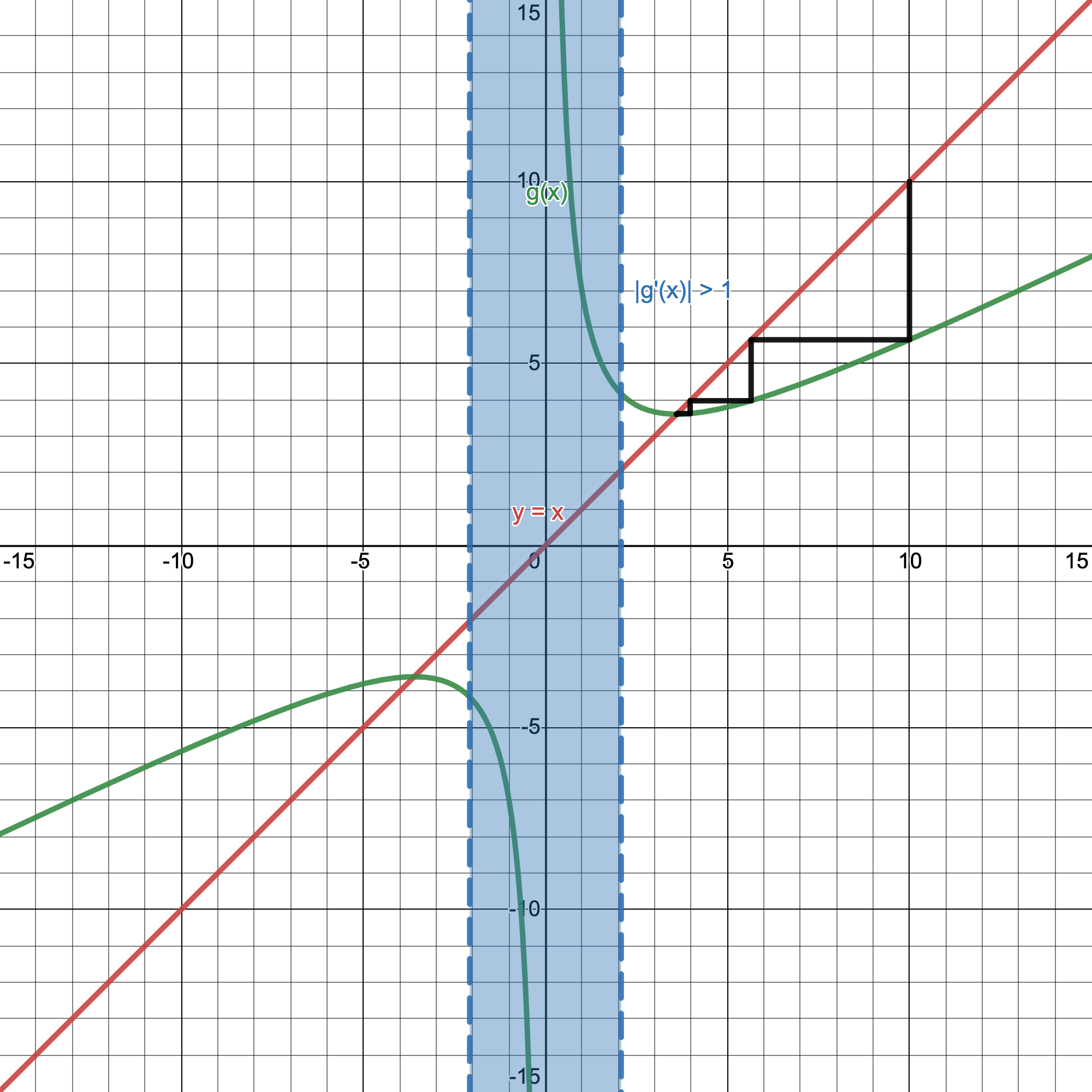
So now we know that for a given $a$, if $|f'(a)| < 1$, it's a shrink, and if $|f'(a)| > 1$, it's a stretch (a negative derivative implies there's also a flip occurring, but we care only about magnitude). You can now kind of imagine what effects these have when we iterate over $f(x)$ for a long time: points will gravitate towards numbers that shrink the area around them, and be repelled away from numbers that stretch them. Now, relating this back to our original Cartesian plot, let's highlight the areas in which $|f'(a)| > 1$.

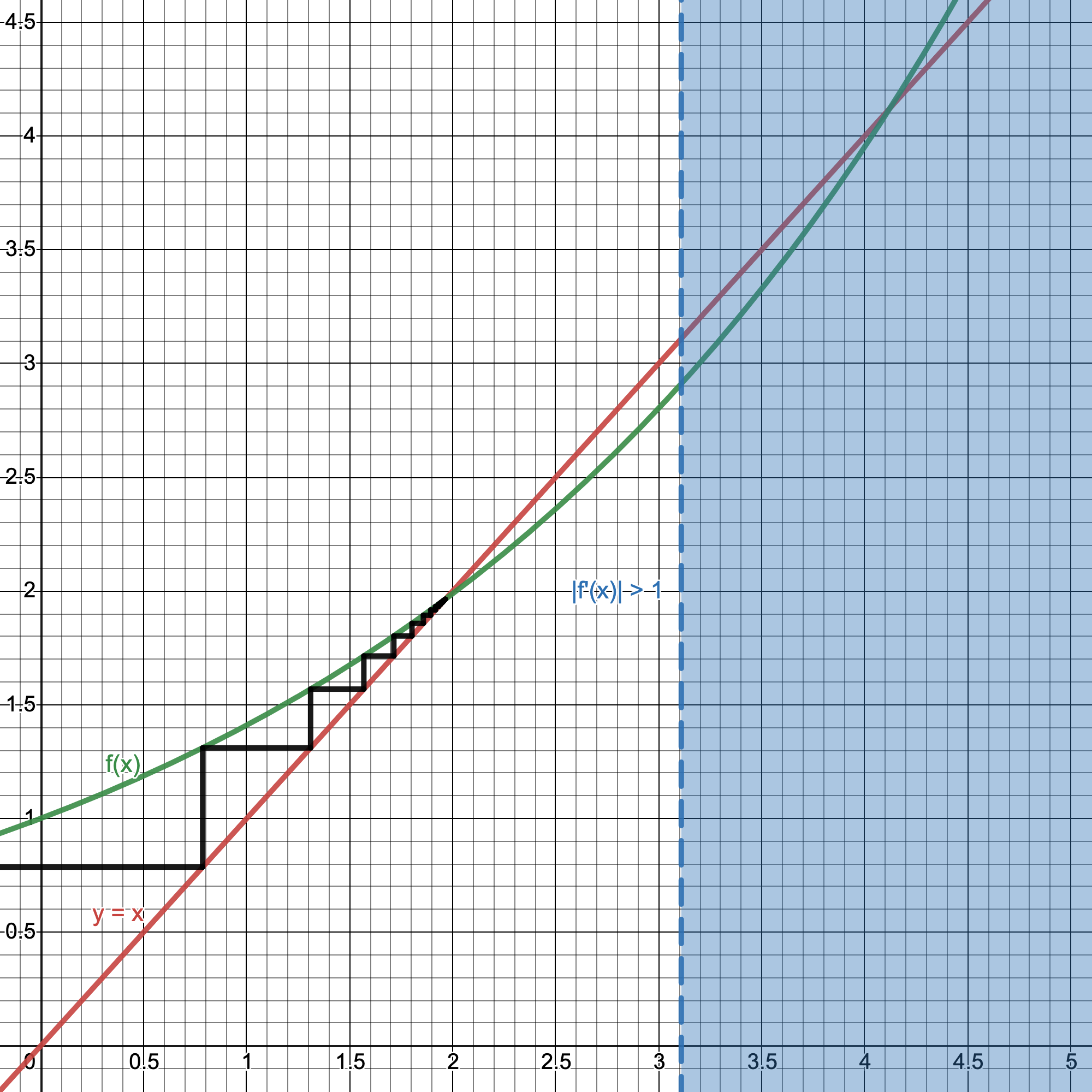
Well, look at that! Our $x=4$ solution is in our blue $|f'(x)|>1$ region, while our $x=2$ solution is not!

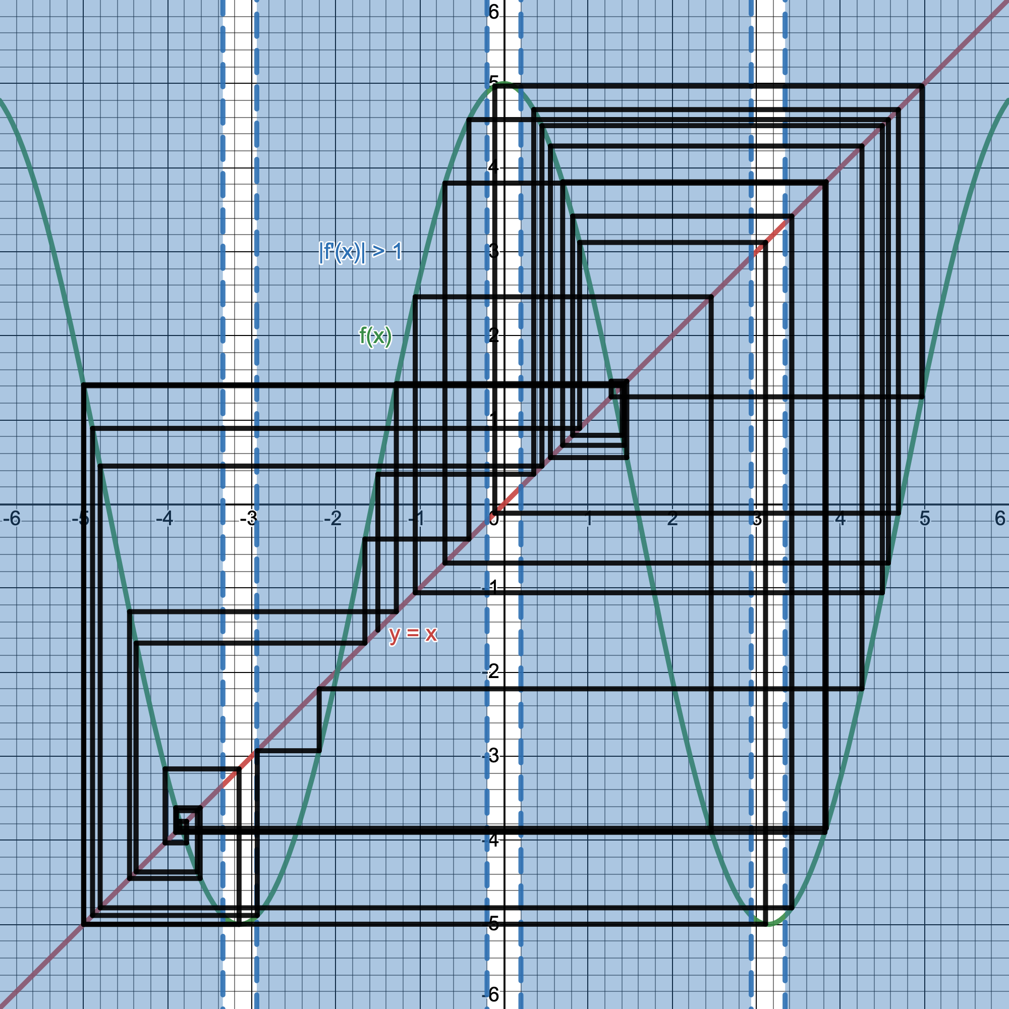
Connecting this all together now, we had two solutions to an iterative function, but only one of which was appearing in practically every case. When graphing its respective cobweb plot, we see that one solution lies in a non-sensitive region ($f'(2) = .6931$), while the other does ($f'(4) = 1.3863$). So what can we say about either solution? Since we know $f(2)$ is not sensitive to small changes and moreover shrinks space around it, we know that $x=2$ is a stable fixed point of the iterative function $f(x) = \sqrt{2}^x$. It's stable under the notion that because it isn't sensitive to small changes in its neighborhood of points, with each iteration we take, we map points closer and closer to $x=2$ due to the squishing effect of its derivative. But for $x=4$, which is sensitive, each iteration tends to stretch and repel points away from $x=4$, even though it too intersects in our cobweb plot as well as analytically solves the equation. Hence, we call $x=4$ an unstable fixed point of the system. Just like we've described, while $x=4$ is valid for its seed value, the slightest discrepancy in value pushes numbers away from it to either start approaching $x=2$, or diverge to infinity (like in our rounding error in the Python script before!). If we quickly go back to our graph style with 2 number lines and perform the function iteratively there, we can really see what these pulls and pushes of numbers looks like. Here's what the first 10 iterations of $\sqrt{2}^x$ looks like:

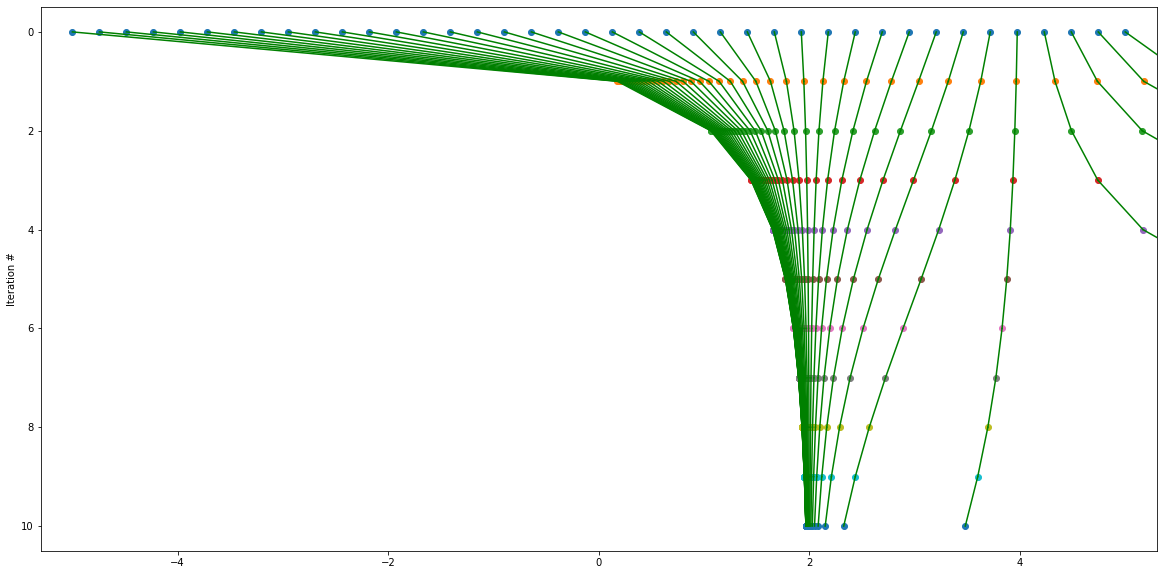
You can really see how tight the points coil around $x=2$, and split away from $x=4$. Even with an initial value that starts so close to $x=4$, you can still see it slightly drift away from it at each iteration. This is why thinking of derivatives as measures of sensitivity is so important: the value of the derivative tells you how strong of a pull or push certain numbers have. Consistent with our findings, $x=2$ has a pulling effect around it with a small derivative, while $x=4$ has a pushing effect with its large derivative.

This is why we were also able to use cobweb plots: they were the geometric algorithm to solve when $f(x)=x$, which makes sense as if something is a fixed point, no matter how many times we apply a function to it, it should remain the same. So when solving $\sqrt{2}^x = x$, you'll get the intersections we found earlier at $x=2,4$ (if you want to try and actually solve this equation, it requires the clever use of the Lambert W-function). That's why we were able to analytically solve for two different solutions, but only one kept popping up everywhere. This isn't limited to just power towers, though.

Variations

This type of relationship between stable and unstable fixed points is everywhere. Take the well-known infinite fraction below:

By setting this equal to $x$, we can solve it just like we did before with the power towers.

Using the quadratic formula, we once again get two solutions:

The famous Golden ratio $\varphi$ and its underrated second solution. Still, it begs the question, how can a completely positive infinite fraction equate to something negative? Illustrating this with our cobweb and sensitivity regions will make this clear once again. Setting $f(x)=1+\frac{1}{x}$, we get…

A lot like $x=4$ when iterating $\sqrt{2}^x$, $1-\varphi$ is the unstable fixed point in the sensitive region, with numbers getting pushed away at every iteration, while $\varphi$ is the stable one which we quickly spiral down towards. We can quickly verify that $1-\varphi$ is a "valid" solution by plugging it into $1+\frac{1}{x}$ just like we did with $x=4$ into $\sqrt{2}^x$.

For its own seed value, $1-\varphi$ is valid, but I guess that's up to you if you want to equate a negative value to a positive infinite fraction.

For those who are interested, try setting your seed value to a number in the form of $-\frac{F_n}{F_{n+1}}$ where $F_n$ represents the nth Fibonacci number. The Golden ratio is closely tied to the Fibonacci numbers, so it may be a bit unsurprising why they may relate here. If you try to iterate over any number in this form, you'll eventually hit a point where evaluating the function becomes undefined. Try plugging in a few and watch the strange cascading effect happen.

There are a whole host of functions that have interesting iterations as well. Let's try $f(x) = \cos(x)$

Since $f'(x) = -\sin(x)$, $|f'(x)|$ is always less than or equal to 1, so all fixed points it has will not diverge. In this case, we get a solution of $\approx .73909$, sometimes referred to as the Dottie number, which has its own set of interesting properties (for one, it's a transcendental number of the likes of $\pi$ and $e$!). If you are interested in a bit of why this has a fixed point, allow me to point you towards the Banach Fixed-Point Theorem for an interesting perspective that guarantees this fixed point. Let's try another function. What happens if we scale $f(x)$? Let's try $5f(x) = 5\cos(x)$

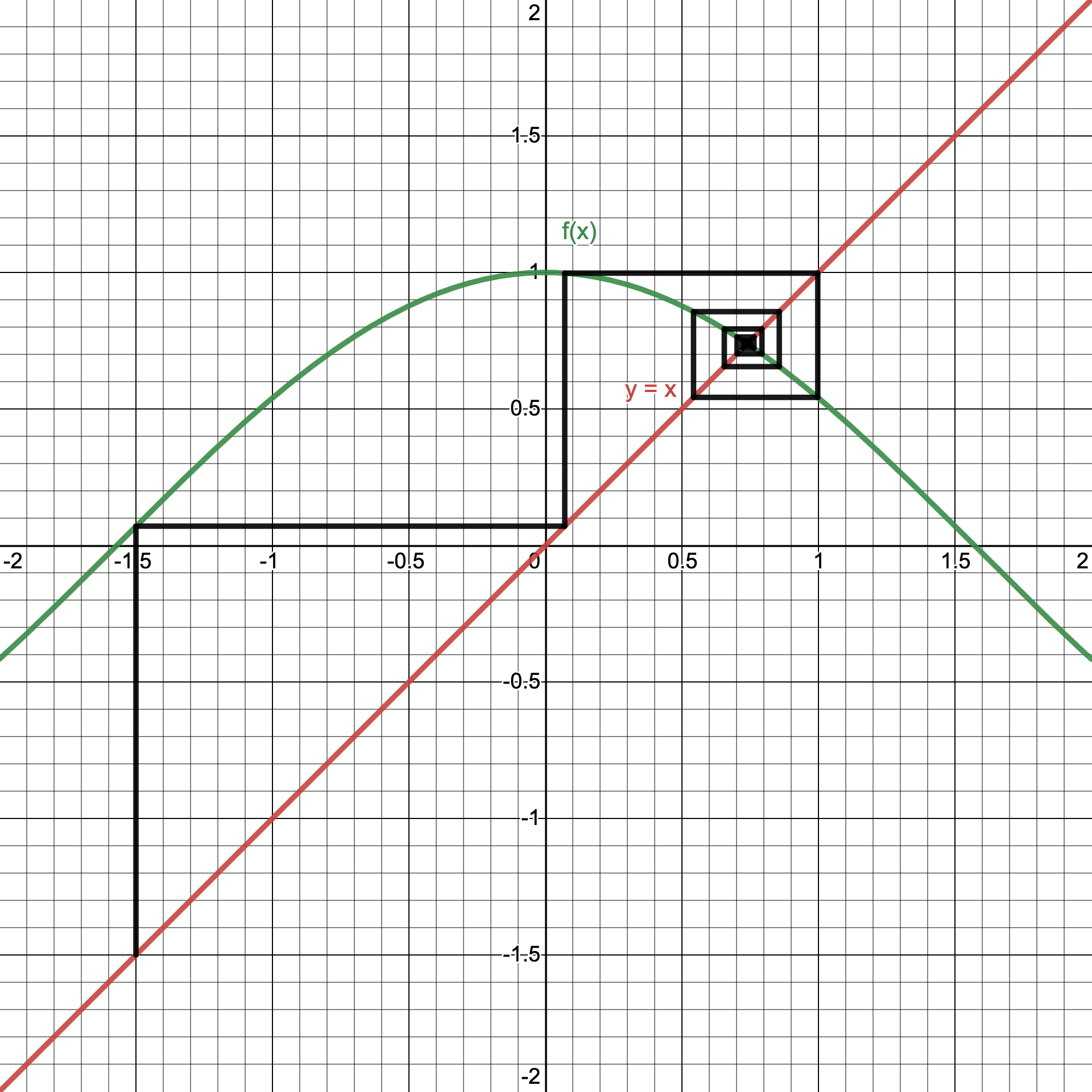
We have not one, not two, but three different intersection points of where $5\cos(x) = x$. But notice, all three of them lie within the sensitive region where $f'(x) > 1$; they're all unstable. You can probably tell just by looking at it, it's a very chaotic diagram. This might not be unexpected for some of you though. If it doesn't converge to anything, but also not diverge, why wouldn't it just randomly jump around ad infinitum? Well, let me just present another function to explain why. Let's make a cobweb plot for $f(x) = 3.2x(1-x)$

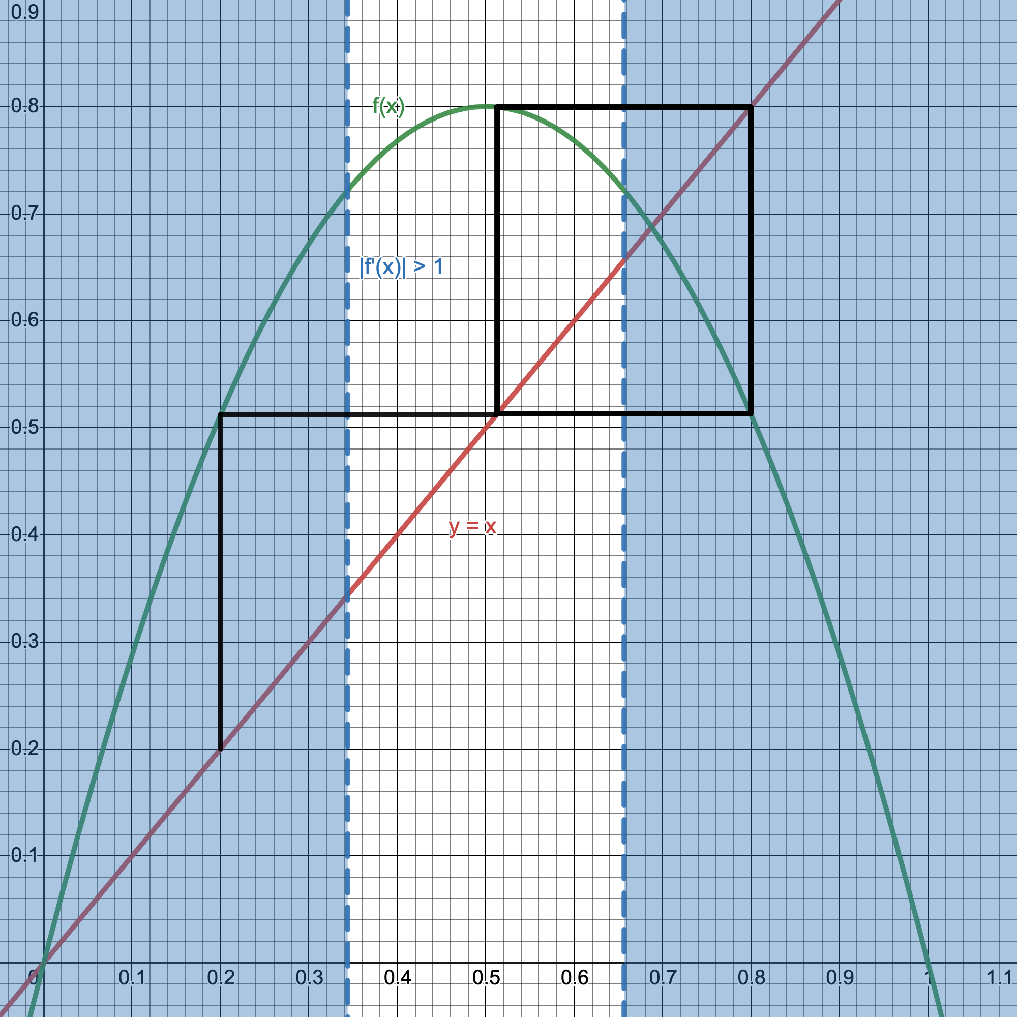
Here we have 2 intersection points, both of which are in the sensitive region where points should not converge to excluding its own value, and that's exactly what we see with no definite attraction to any one fixed point. Yet, it's not like our iterations are randomly moving. In fact, just looking at the diagram, it's quite predictably going in a cycle between two $x$-values of $\approx .516$ and $\approx .8$. The difference between $5\cos(x)$ and $3.2x(1-x)$ is how it interacts with our seed value. For the former, it has a quality known as sensitive dependence on initial conditions, or more commonly referred to as the Butterfly effect: a small change in the seed value can produce wildly different outputs in iteration in the long run, just like how a butterfly's wings can produce a hurricane years later halfway across the globe. This is a common property of what is aptly deemed chaotic behavior. The latter function, while it may not have a convergent value, it does not exhibit Butterfly effect-esque behavior nor chaos while iterating over it, and instead settles into this cycle. As a kickstarter for those interested, $3.2$ in the latter function was not an arbitrary choice: it comes from a family of iterative functions of the form $rx(1-x)$ known as the logistic map. There's so much to talk about there, it likely will be its own post later, but that's for another day.

I want to go back to the Golden ratio problem as there's a neat extension to a more general case of an iterative approximation technique that can be more applicable to problem solving that I want to share. It is known as the Newton-Raphson Method which can (usually) effectively hone in on roots of a polynomial quite efficiently.

Newton-Raphson Method

The idea is fairly similar to what we did before, but since it's catered to finding roots of polynomials, its iterations have a modified step as we're looking for intersections with the $x$-axis instead of the line $y=x$. Here's the basic idea: 1) Pick an initial seed value $x_0$. 2) Draw a vertical line (like we did with the cobweb) until we hit the function $f(x)$. 3) Draw the tangent line of $f(x)$ at $x_0$, and see where it hits the $x$-axis. Call this new point $x_1$. 4) Repeat the process as many times as you'd like for as accurate an approximation as you'd like up to some $x_n$. Here's an example geometric interpretation for this method with $f(x) = x^2 - 13$.

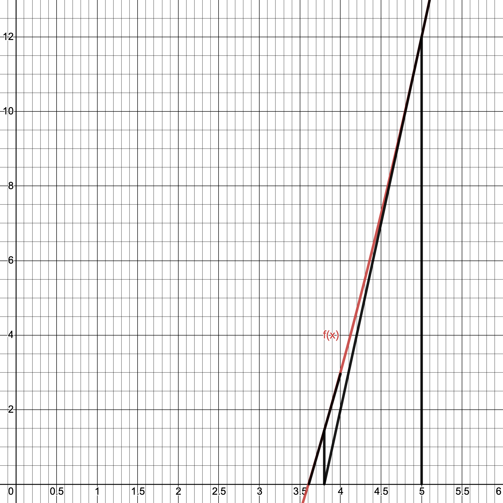
I had to zoom in extremely close for this graph because, as you can see, just after two iterations from a seed value $x_0=5$ finds a really accurate approximation of one of the roots of $f(x)$ and you wouldn't be able to see those lines unless magnified by this much. Let's work out a general iterative formula for this method. We first start with some $f(x)$. Just by using derivatives and definition of a line passing through the point $(x_n,f(x_n))$ for our tangent, we can solve the equation

to find the next point $x_{n+1}$ to continue iterating on (as it should be the $x$-intercept of that line like the instructions describe). Doing some basic algebra shows that:

So, tidying things up, for a given (continuous and differentiable) function $f(x)$, we can approximate its roots by iterating over with some initial $x_0$:

Trying this out with our $f(x) = x^2 - 13$, our recurrence relation after some simplifying becomes

Or if you liked our previous notation, we can rewrite this as a function and iterate over

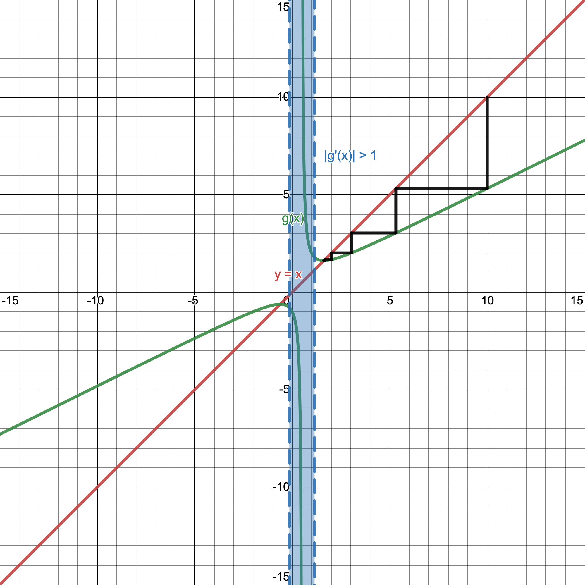
Since this is in function form, we can use our old friend the cobweb to solve this for us.

It nicely finds $\sqrt{13}$ as a solution, just as we would expect. However, notice that there are two intersection points that lie outside of the sensitive region. One we found at $x=\sqrt{13}$, and the other is actually the second solution to $x^2-13=0$ at $x=-\sqrt{13}$. Our seed value significantly matters more in this case, as now depending on which zero of $f(x)$ is closer, our iteration will target only the closest solution, and this only becomes more important the more zeroes our function contains.

Even with all those caveats, notice what we just made! Our iterative function $g(x)$ is essentially a square root estimator, but with no exponents! While it's nice and convenient just to use exact answers, having decimal approximations are just as useful, especially for computers who don't have unlimited memory to use exact answers. For any number $n$, we can calculate $\sqrt{n}$ as accurately as we'd like by iterating over the function

as many times as we want. There are some exceptions where certain seeds can infinitely cycle or actually result in no subsequent $x_{n+1}$ (imagine a horizontal tangent line), but this method is incredibly useful, as this doesn't just extend to square roots, but to any function you want to approximate using the aforementioned formula

Here are a few other iterative functions for other roots of $n$:

Going back to our Golden ratio iteration, we can rewrite it under the fixed point formula $f(x)=x\rightarrow 1+\frac{1}{x}=x$. If you multiply that through by $x$ and rearrange, we get a quadratic $x^2-x-1=0$. That's a quadratic we can solve for with the Newton-Raphson Method! Plugging it into the formula, we get a function to iterate over as

And sure enough, it works! The advantage of using the Newton-Raphson Method in this case, is that we no longer have to worry about unstable fixed points, as all of our solutions lie outside the sensitivity region. So even if we lose some insight into the nature of each solution, we consistently find each solution of $\varphi$ and $1-\varphi$ to an accurate decimal expansion with the right seed.

What Else?

Iteration and fixed points become one of the prime topics for dynamical systems and describing much of the world around us. We discussed the Newton-Raphson Method of root finding, but there are many other recurrence relations for approximating roots of functions, each catered for their own purpose with different convergence rates and fail cases. Moreover, this is just a single use of the Newton-Raphson Method, for it is more well known as an alternative to gradient descent. Solving systems of differential equations comes down to finding the equivalent of a higher-dimensional fixed point, or in other words, an eigenvector: a vector (which is just an object that can encode more than one number and hence dimension) which doesn't change direction under the transformation describing the system of equations. Markov chains are also another extremely important occurence of fixed points over iteration: after a long series of transitions between states, we can make an overarching statement about the system as a whole reaching an equilibrium state where transition probabilities are expected to remain the same (going back to that idea of eigenvectors!). Synchronization is a prime example of a fixed point under iteration: even if a group of fireflies begin out of phase with one another, their coupling over time will reduce each other into a single large group with one cyclic, uniform behavior. The Mandelbrot set (and all of the Julia sets, for that matter) arise out of the fact that some complex numbers are bounded under iteration of functions $f(z)=z^n+c$ that remain bounded after a long time (sometimes being bounded to multiple values at once!). There are even entire studies dedicated to this. Invariant theory studies mathematical groups and polynomials to see how they remain unchanged under transformations. Almost all of chaos theory is about stability (or the lack thereof) over long periods of time (Nicky Case has a great introduction to attractors), and especially when what should be simple, predictable equations are not (we already talked about the logistic map, but see it illustrated in the Bifurcation diagram. It is particularly interesting for it appears in the most unlikely of places). We saw some chaotic behavior earlier, and the way I deduced it was chaotic was with a quantifier all iterative functions and maps have known as the Lyapunov exponent, and this itself is so interesting to look at for how functions change in behavior along with its Lyapunov exponent. For fixed points alone, there are hundreds of theorems dedicated to analyzing them (most notable of them being Brouwer's Fixed-Point Theorem).

If you are interested in anything covered here, popular math YouTube channel 3Blue1Brown made not one but two videos discussing this idea of derivatives and infinitely stacked operations with the exact puzzle I posed at the start of this post. Their first video is what originally inspired me to look into these objects more when I first saw it a couple yeas back. Their animations do wonders compared to what any text post can do, so please do check them out if you want a more visual approach to these processes along with some additional justification for solutions to iterative processes.

Fixed points appear everywhere, and I hope this shared a few insights into how they can appear, deceive, and approximate even the most out there of expressions.