Delta Thoughts

Today, I want to talk about a really powerful tool in math and statistics, that on its own may seem very niche, the concept behind it is something really—and I mean really—powerful and is how many other discoveries and tools are made and immortalized. In particular, I want to talk about the Metropolis-Hastings algorithm and Markov chain Monte Carlo methods. If you want to skip the basics, here's a short table of contents:

1. Markov Chains
2. Monte Carlo Simulations
3. The Metropolis-Hastings Algorithm

Brief summaries are at the bottom of each section if you want a quick referesher for anything above, but first, some review.

This is also all written more formally with other examples in this paper.

Markov Chains

Markov chains, in essence, are a way to model a process that randomly jumps between different outputs, where each output is said to have some probability to jump to other outputs. They're sort of like rolling dice, but the likelihood you roll any number is only dependent on the number you rolled last. It might help to describe this with an example. Let's say you want to know what the weather will be in 5 days: will it be sunny or rainy? Fortunately, the weather doesn't vary too much, so if it's sunny one day, it's likely to be sunny again the next day with 80% chance. If it's rainy, it will likely be rainy again too, with, say, 60% chance. This can be shown quite succinctly in a little diagram:

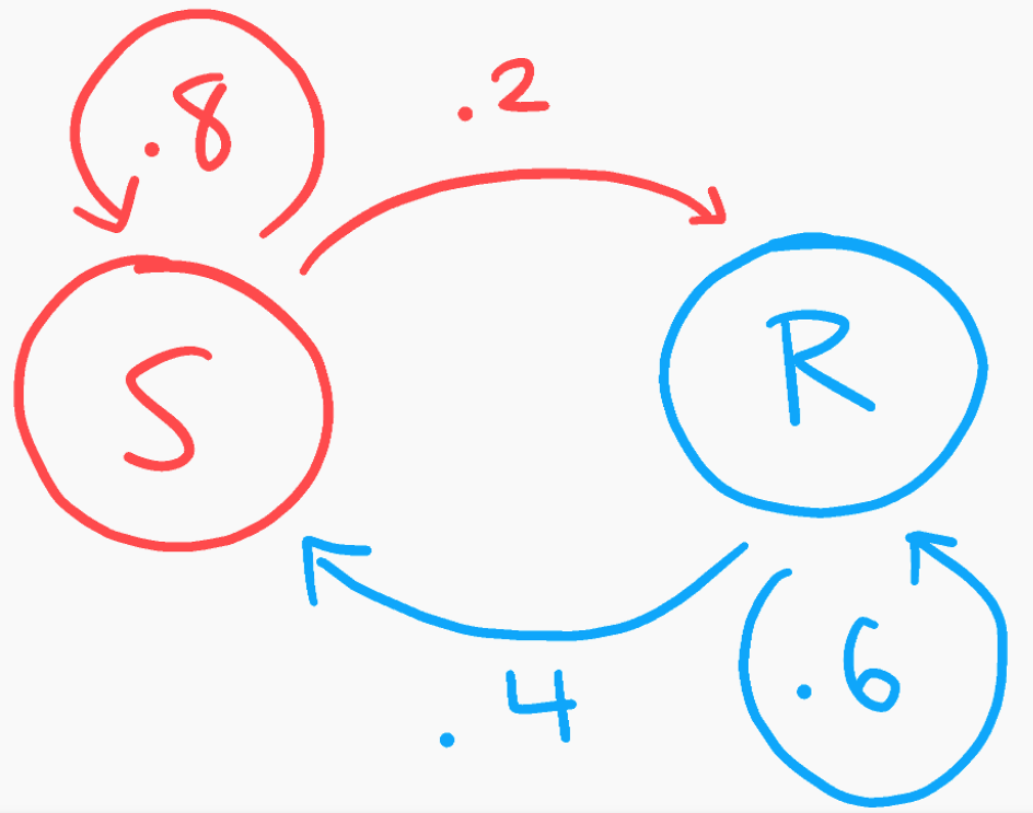
This is our actual Markov chain, showing the two transition states, S(unny) and R(ainy) with their associated transition probabilities. However, we can't actually do much with just a picture alone. So, we can rewrite these probabilities and encode them in a matrix:

You can think of each row as a different state for current weather, and the columns as probabilities for different states of tomorrow's weather. In this case, I have written row 1 and column 1 to indicate sunny days, and row 2 and column 2 to be rainy days. That's why entry $a_{1,1}$ in row 1, column 1 shows 80%, because if it is sunny today (row 1), we expect an 80% chance for it to be sunny tomorrow (column 1). Similarly $a_{2,2}=.6$, as if it's rainy today, we expect a 60% chance for rain again. $a_{1,2}=.2$ means that if today is sunny, then there is a 20% chance of rain tomorrow, and for completeness sake, $a_{2,1}=.4$ indicates a 40% chance for it to be sunny given today is rainy.

What we've built here is known as a transition matrix, as, well, it's a matrix that shows transition probabilities; it's a matrix that shows how likely we are to jump from one state to another. In this case, our states are the different weathers: sunny or rainy. So, how does this help us answer our original question of the what the weather will be in 5 days? Well, let's first try to find the weather 2 days from now. We know how to model 1 day from now, and since these are probabilities, wouldn't it make sense just to multiply our matrix by itself?

Our probabilities have changed a little bit. Now it's saying, if today is sunny, there is a 72% chance it will be sunny 2 days from now. The reason why multiplying our matrix itself to get this result makes sense is because of the mechanics of matrix multiplication essentially asks: "What is the probability from getting from one state to another in two steps?" If you work out the multiplication itself, it might be clearer, but the way I like to think about it is in terms of transformations of space. For those familiar with a bit of linear algebra, we can think of our matrix $M$ as a collection of basis vectors that scale space (where our vectors in space can be thought of as a collection of starting states, i.e. the initial observed proportion of sunny days to rainy days). So applying $M$ once transforms space, we can then take that as a new "default" or "unit". If we apply $M$ again to our basis vectors, it has the effect of transforming space once again. This can be thought of as our standard, independent probability multiplication, but instead of changing a singular probability (i.e. dice value), we are changing two (likelihood of sunny and likelihood of rainy days).

With this in mind, our question is easy. It boils down to what $M^5$ is.

So if today is sunny, we look at row 1 and can expect a 67.008% chance of sunny weather, and if it's rainy, row 2 shows a 65.984% chance for sunny weather. Nice! But you might be looking at that matrix and notice that row 1 and row 2 are almost the same. Watch what happens if we don't check for any 5 days in the future, but if we look towards an infinite number of days ahead?

The rows do become the same. So, if we were to pick a random day far, far into the future, we can expect it to be twice as likely to be sunny than rainy regardless of today's weather. There's two important interpretations of this fact. 1) going back to our transformation of space idea, this equilibrium state is our eigenvector (specifically for $\lambda=1$) of our transition matrix $M$. Meaning, it is the solution to the matrix equation $vM = v$ where $v$ is a row vector (here, $v=\begin{bmatrix} .\overline{666} & .\overline{333} \end{bmatrix}$). The second—and more important—way to think of this equilibrium state is that it is the final, or stationary distribution of sunny and rainy days. That is, if you took the fraction of $\frac{\textrm{Sunny Days}}{\textrm{Total Days}}$, you'd expect it to approach $\frac{2}{3}$ as time went on, and $\frac{\textrm{Rainy Days}}{\textrm{Total Days}}$ to likewise approach $\frac{1}{3}$.

To summarize, here are a few important concepts about Markov chains:

1. A Markov chain is a random process that describes the ability to switch between multiple states.
2. A Markov chain's probability for any future state depends only on the current state (this is also known as the Markov property).
3. The sum of each row of a Markov chain's transition matrix must sum to 1 (something has to occur at each time step for each state, even if that means not changing states)
4. All Markov chains will eventually reach an equilibrium state that describes the final distribution of states over a long time.

Markov chains are extremely powerful tools to model dynamics with multiple states due to their above properties, but some of their uses from chaos to disease modeling deserve their own post another day.

If you understood this so far, you've got the hardest part of Markov chain Monte Carlo methods under your belt. That being said, we are still missing second MC of MCMC.

Monte Carlo Simulations

Monte Carlo simulations are probably the closest you'll ever get to the scientific version of guess-and-check. The idea is if there is something that's too hard to calculate, you do a bunch of mini, random experiments to obtain data that can give us numerical approximations. It's very akin to Bayesian thinking: the more data you give to your approximation, the better the you can "update" your approximation to be more accurate and confident. As with all things, let's do a quick example.

If I hand you a coin, you probably would assume it's a fair coin: 50/50 chance for either heads or tails. But how could you verify that it is indeed a fair coin? Well you could flip it and see what it turns up as. Heads! "It must be an unfair coin as it flips heads 100% of the time!" said no one ever. Of course a single data point isn't nearly enough to draw any conclusions, so you need to flip it again. Heads again! Definitely weighted, right? Even if you get only heads twice in a row, that still isn't conclusive. You need to flip the coin a lot of times. By a lot, upwards of hundreds for a reasonable guess at the balance of the coin, and upwards of thousands for an ideal approximation. For all you know, those first 2 heads could be in a much larger sequence of flips you have yet to unfold:

Just like that, our coin reaches that 50/50 split significantly closer within just a few additional flips.

Each one of our data points were flips in this case, and we call those data points samples. The important part to note, though, is that there is a sense of randomness in each sample. The idea behind a Monte Carlo simulation is that even if our sampling method is random, the more samples we take will average out to the true value (think the Law of Large Numbers). The is why the more samples we take, the more accurate our estimations become. This is a lot like unbiased sampling in research studies: you can't reasonably survey everyone in a population, so you take a smaller, random sample in the hopes that it will be representative enough to make reasonable conclusions of the larger population.

Again, just to summarize a few details:

1. Monte Carlo simulations use random sampling to get numerical estimations for hard to otherwise calculate results.
2. The more samples/trials we take, the more accurate our results.
3. While taking more samples is more accurate, it also become less efficient to compute and gather results, so you have strike that balance between more accurate results or quicker results.

With all that out of the way, let's put it all together into one cool algorithm.

Metropolis-Hastings and MCMC

So far, we've sampled from relativiely easy things to run trials on and get samples. Flipping a coin and rolling a dice are nice distributions to run trials on are they both can be modelled by a nice uniform distribution (even for weighted dice/coins by partitioning the uniformness). This is due to the niceness of a discrete distribution where there is only a finite number of results our black box can output. Often the case, we have a continuous function where we don't have probabilities for individual results, but rather a range of results. To get the gist of it, take the uniform probability distribution between $[0,1]$. What's the probability that you pick $0.235326…$? Obviously, out of an infinite amount of possibilities, a single, specific number to pick is probability 0. BUT, the probability of picking a number between $[.25,.75]$ is exactly $.5$, as we're picking from half of our total range. This is the idea of probability density. So, you can imagine for more complicated distributions (especially those taken from real life data) can be a lot more difficult to get samples from, or properly know the densities of regions. Here's where our MCMC comes from.

Markov chain Monte Carlo methods combine two important aspects of the two concepts the name implies: a Markov chain's equilibrium distribution and Monte Carlo simulation's random sampling. Here, we make a Markov chain who's stationary distribution is equal to our hard-to-model probability distribution by doing a random walk around the distribution (for the sake of notation, we'll call our "target" distribution we're trying to model $\pi(x)$). In this case, we do so with the Metropolis-Hastings algorithm which is extremely simple:

1. Pick a starting point $x_0 \rightarrow$ this is the start of our "walk". An initial sample, if you will, that we provide ($x_t$ means our current sample at time $t$).
2. Now pick a new, random point $y$. Call $y$ the "proposed state" for $x_{t+1}$.

3. See how "good" $y$ is compared to $x_t$.

   i. If $y$ is "better", we let $x_{t+1}=y$

   ii. If $y$ is "worse", we might let $x_{t+1}=y$, but not always.

4. For $t=1,2,3,…$, repeat steps 2 and 3.
5. Profit.

This is extremely vague, but I intentionally left it as such, because often times the formulas can confuse the language. In essence, this is what Metropolis-Hastings does to generate samples. We take a sample $x_t$ at a time $t$ that "traces" our distribution, and as $t$ gets larger, the more accurate our "trace" of the curve we walk around gets better. Let's put some of the formulas back into the instructions above and go at it one step at a time.

Step 1 is easy enough: we give any number for our algorithm to start with. Literally anything. You can give smart guesses that speed up the process, but that will be clear in a second.

Step 2 we don't actually perform, but rather design. Unlike Step 1 where we gave some determined number of our choosing, Step 2 we implement a transition kernel to pick a step for us. This kernel is a function $Q$ that takes a current spot $x$ and with some probability outputs a new spot $y$. That is, $Q$ is a distribution that randomly generates a new point $y$ given a current one $x$, which we will write $Q(y|x)$. This is how we make our "proposed state" and how we actually implement our walk. You may be wondering though, "What actually is $Q$?" Well, that's up to you to decide! Since $Q$ itself is a distribution around our current state $x$, you can shape $Q$ in whatever way you want! In general, though, it's not too important, but spending time to design a specific kernel can optimize and speed up the process.

Step 3 is our "goodness" check. Once we have a proposed state generated by $Q$, we need to see if this proposed state is in a more "likely" or dense spot on our distribution $\pi(x)$. The idea is we want to generate samples representative of $\pi(x)$, so it should be obvious that we should visit the probabilistically more dense spots, a.k.a. visit the spots the distribution says is more likely. Geometrically, this is a point higher on our distribution curve.

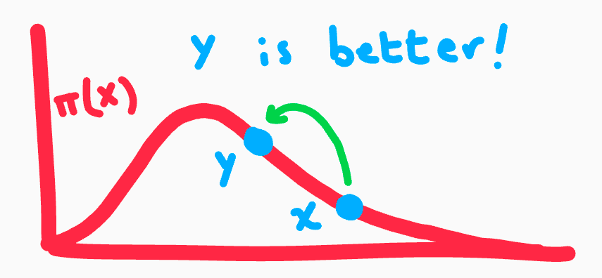
But remember, just because $y$ is not better doesn't mean that we outright reject it. We instead accept it with probability proportional to how much worse it is. If $y$ is half as high as our current spot $x$, we flip a coin and might accept it with 50% probability. If $y$ was a third as high $x$, we flip a weighted coin and might accept it with probability $\frac{1}{3}$. In other words, we can write our acceptance probability $A=\min(1, \frac{\pi(y)}{\pi(x)})$. If $y$ is higher than $x$, or $\pi(y)>\pi(x)$, then $\frac{\pi(y)}{\pi(x)} > 1$ and we accept it outright. If $\frac{\pi(y)}{\pi(x)} < 1$, then we accept it with probability of that fraction.

This acceptance probability is also what makes this algorithm so good: we only need to know our target distribution $\pi(x)$ up to a constant! If $\pi(x) = c\cdot P(x)$, then our acceptance probability would be $A=\min(1, \frac{c\cdot P(y)}{c\cdot P(x)})$ which simplifies to $\min(1, \frac{P(y)}{P(x)})$, making the constant irrelevant. This is ideal for real life experiments as perfectly measuring constants from observation can be very difficult.

Steps 4 and 5 are pretty self-explanatory, so just to rewrite it more formally, here is the whole algorithm one more time:

1. Pick a starting point $x_0$.
2. Sample a new proposal state $y$ with probability $Q(y|x_t)$

3. Compute $A=\min(1, \frac{\pi(y)}{\pi(x_t)})$.

   i. With probability $A$, accept our proposed state and let $x_{t+1}=y$

4. For $t=1,2,3,…$, repeat steps 2 and 3.

5. Profit.

However I must admit, I did lie to you, but only a little bit. The acceptance probability I gave is actually for the Metropolis algorithm, not the Metropolis-Hastings algorithm. The acceptance probability for the Metropolis-Hastings algorithm is $A=\min(1, \frac{\pi(y)Q(x_t|y)}{\pi(x)Q(y|x_t)})$. This is because the Metropolis algorithm only works when $Q$ is a symmetric distribution, meaning that $Q(y|x_t)=Q(x_t|y)$, which returns us to our familiar fraction from before. MH allows asymmetric kernels to speed up the algorithm, but otherwise the concept is the same.

With 5 very simple steps, we are able to take samples from continuous distributions just like that! The Monte Carlo aspect is pretty obvious with the random steps with generating random "proposal states" $y$ in Step 2. The Markov chain might be a bit more concealed, as we never actually explicitly define it. But, look at Step 3 again, as that resembles something very close to our transition probabilities before. Step 3 is actually our Markov chain implicitly defined! Since there are an infinite number of states/values to pick and another infinite number of states to transition to, we can't define an infinitely sized transition matrix. So, instead, we define transition probabilities as needed with our kernel $Q$. And notice, our kernel maintains the Markov property as each proposed state only relies on the current. This is because we sort of reversed the way we defined our Markov chain! In our weather example with sunny and rainy days from above, we defined transition states and the stationary distribution followed suit, almost like property or characteristic of our Markov chain. Here, our Markov chain is instead defined by the fact we want our stationary distribution to mimic $\pi(x)$. This is why we don't outright reject states that are less "good" in our acceptance probability, but rather accept it proportional to how less "good" it is as that will reflect our distribution's shape.

But just like in our original Markov chain example, it's not perfect immediately. Notice in our original weather example with sunny and rainy days, 2 iterations with $M^2$ was no where near close our stationary distribution, and while 5 iterations at $M^5$ was closer, it still was nowhere near ideal. You have to burn in some states before proper, accurate samples can be generated.

Here's some short Python to implement the Metropolis-Hastings algorithm to estimate the following Laplace distribution:

Here it is in only 20 lines of code:

import numpy as np
import matplotlib.pyplot as plt

def target(x):
  return .5 * np.exp(-abs(x)) # Target distribution π(x)
def accept(p):
  flip = np.random.uniform(0,1)
  return p >= flip
def metropolis(iterations):
  states = [] # Samples generated by the algorithm
  # Step 1 --> initialize an x0
  current = 1 
  for i in range(iterations):
    states.append(current)
    # Step 2 --> Q generates a proposal (normal distribution)
    proposal = np.random.normal(current, 1) 
    # Step 3 --> Check how good our proposal is
    goodness = min(1, target(proposal)/target(current))
    if accept(goodness): 
      current = proposal # If we like the proposal state, we jump there!
  return states

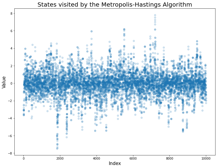
Here is the scatter plot of our algorithm walking all around $\pi(x)$ across 10000 iterations...

...and here is the corresponding histogram that fits almost too perfectly to our target distribution.

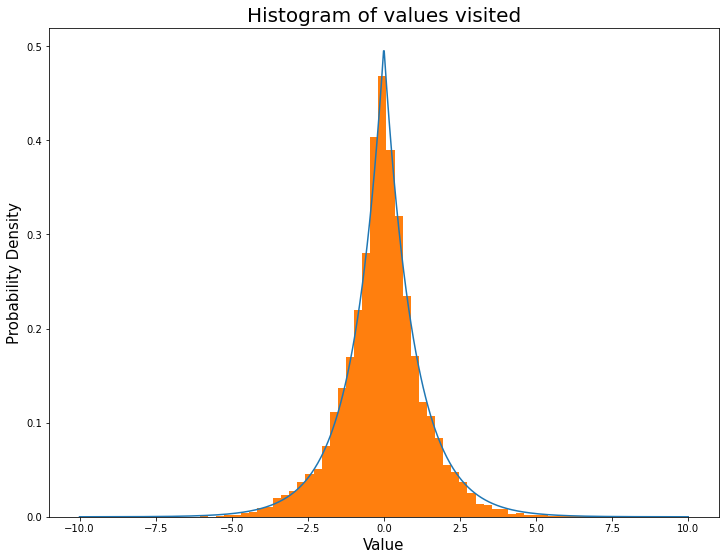
We can now generate discrete samples proportional to our continuous distribution!

The algorithm aside, an extremely important concept is shown here: reframing questions and objects and asking them from a different perspective can lead to extremely powerful tools and thoughts. We take a Markov chain, and instead of letting its equilibrium state arise as a property, we use it to turn our definition inside out and use the equilibrium state itself to define the Markov chain. This pattern of rethinking concepts has always been a useful, sobeit from building intuition while learning, to defining tools in all of math. From connecting why Mandelbrot set to its cardioid and cycloids, to encoding parameters in 4-dimensional space means, to even Fourier rebuilding functions from sine waves, the most impactful question one can ask is usually in the form of, "What if?"