Last post, we looked at different types of billiard problems, a class of math problems analyzing how light bounces with different setups of mirrors. Notably, we saw how straight lines make for very simple, easy to compute mirrors, while others like circular ones, can be incredibly frustrating.
A large portion of last post's content, though, was made up of interactive graphics. While I went over much of the math that goes into solving these types of problems, we skipped over a large part of the math that goes into simulating them. Math is very nice in that many problems can be solved with nothing more than a pen, paper, and your mind, but oftentimes, that's only helpful if you are confident in how to approach the problem. What computer's can do is help build our intuition to solve a problem by calculating, drawing, and modelling scenarios with precision and speed we can only wish to achieve.
So, today, we'll look at some of the clever math that goes into computer graphics (that we'll later extend), and to introduce such a topic, we'll look at a simple, fundamental problem in graphics: how do you find the intersection between a line and a circle?
Languishing Lines and Confounding Circles
Before we can even attempt this problem, we're going to have to start from scratch, since we have one slight issue: a computer has no idea what a line or a circle is! So before we can do anything, let's teach our computer how to draw a line.
Perfect Parameterizations
At its core, computer graphics is displaying a set of pixels with certain colors. If we want to visualize anything on a computer screen, we just need to find all the relevant pixels (coordinates) to light up and color. Because we want to compute these individual coordinates of, say, a line or circle very quickly and easily, almost always we will use vectors. These can be typical column or row vectors you see in linear algebra, or it can even take the form of complex numbers. The reason why these tend to be helpful is that they give very easy ways to compute coordinates for lines, circles, and other shapes.
If we want to draw a line with slope, say 2, we need to ensure that it is constructed by a vector of slope 2. An easy one to find is the vector $v=\small{\begin{bmatrix} 1 \\ 2 \end{bmatrix}}$ since we know that will pass through the point $(1,2)$. So, to get other points beyond this vector, we can scale $v$ by a factor of $t$ to get other vectors (i.e. points) with the same slope. If $t=2$, we get the point $(2,4)$. If $t=1.5$, we get the point $(1.5,3)$. If $t=239470$, we get the point $(239470,478940)$. Whatever you choose $t$ to be, our vector $v$ will give us a point on the line $y=2x$.
However, this isn't super helpful, since we are still only restricted to lines that go through the origin at $(0,0)$. So, we can add a starting point $\color{red}{p}$ to our vector equation to offset the line by $\color{red}{p}$, guaranteeing our line goes through the point $\color{red}{p}$ (since that's the coordinate generated by $t=0$).
Now we just plot every point for $t \in (-\infty, \infty)$, and we get a line with $v$ dictating the slope of our line (negative $t$ values gives us coordinates behind $\color{red}{p}$)!
Our parametric line $l$ going through point $\color{red}{p}$. Drag the point to adjust it's position.
We can do a similar process for a circle. To parameterize a circle, we'll have to pull from trigonometry. We know that a circle is defined by $x^2 + y^2 = r^2$. The Pythagorean identity tells us that $\cos^2(\theta) + \sin^2(\theta) = 1$, so we can quickly make the connection that $x=r\cos(\theta)$ and $y=r\sin(\theta)$ (which the geometry justifies). This precisely defines $x$ and $y$ in terms of the parameter $\theta$! Again, though, this is centered at the origin, so we can center the circle around a point $\color{blue}{q}$ by adding it to our parameterization.
where $r$ is some real number for the radius of the circle, and $\theta \in [0, 2\pi)$. We can now easily draw both lines and circles!
Now we also have a circle centered at $\color{blue}{q}$ too. Drag the center point to change its position, and the radial point its radius.
Collisions and Intersections
Now that we have defined our line and circle for our computer to interpret, we can start thinking about how to detect collisions between a line and a circle.
Discerning Distances
A good place to start is by looking at how far away the line $l$ is from the center of the circle $\color{blue}{q}$. For reference, the distance from a point to a line is the shortest (i.e. perpendicular) distance from the point to the line. If $l$ is more than a distance of $r$ away from $\color{blue}{q}$, then we know that it's outside the circle and doesn't intersect, and if $l$ is less than a distance $r$ away from $\color{blue}{q}$, then we know it's inside the circle and does intersect.
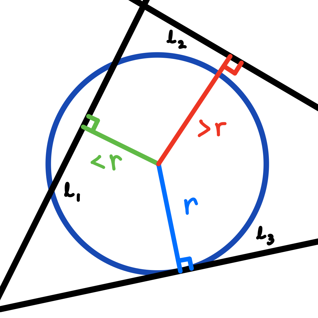
$l_1$ is a distance less than $r$ away from the center, and clearly intersects the circle. $l_2$ is a distance greater than $r$ away, and clearly does not intersect the circle. $l_3$ is exactly a distance $r$ away, making it tangent to the circle (1 intersection point instead of 2).
Let's look at an individual line and see if we can draw any useful conclusions about this distance.
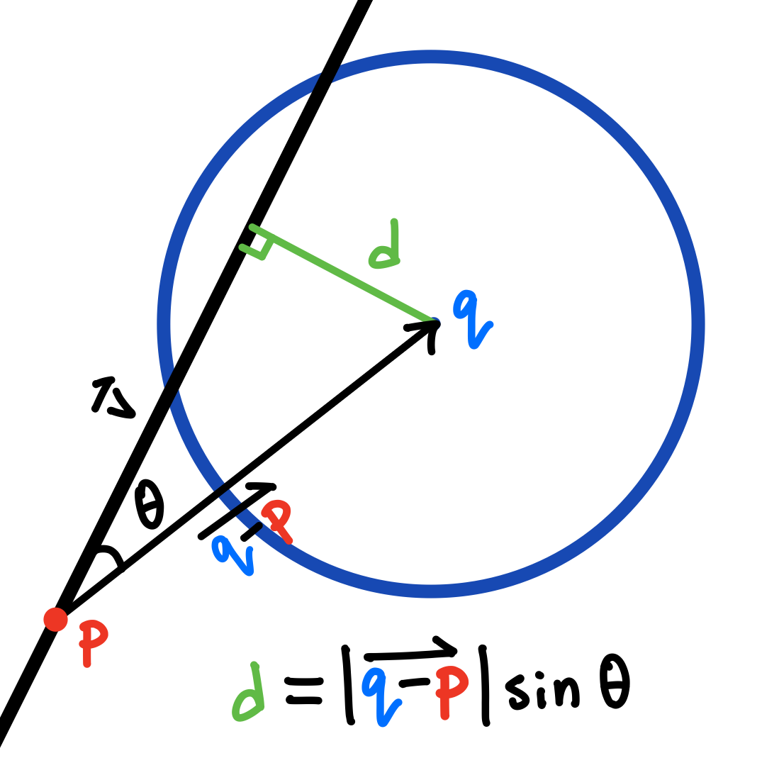
From a given point $\color{red}{p}$ on our line $l$, we can find a new vector between $\color{red}{p}$ and the circle's center $\color{blue}{q}$ as $\overrightarrow{\color{blue}{q} - \color{red}{p}}$. This will form some angle $\theta$ with $l$, more specifically its vector $v$. Recalling that $\color{green}{d}$ is the perpendicular distance between $\color{blue}{q}$ and $l$, we have a right triangle that gives us that $\color{green}{d} = |\overrightarrow{\color{blue}{q} - \color{red}{p}}| \sin \theta$.
If you're familiar with your linear algebra, this almost looks like the formula for the magnitude of the cross product: $|v \times u| = |v||u|\sin \theta$. So, writing our two relevant vectors and rearranging we can see that…
$|\overrightarrow{\color{blue}{q} - \color{red}{p}}| \sin \theta = |\overrightarrow{\color{blue}{q} - \color{red}{p}} \times \frac{v}{|v|}|$
So all we need to do to see if our line intersects our circle is if that cross product is less than or equal to the radius of our circle (if you're concerned about the dimensionality of our vectors—cross products only exist in dimensions 3 and 7—we can treat them as 3D vectors with z-component 0, which makes the calculation easier and equivalent to the determinant).
If this isn't totally apparent why this is true, it has to do with the geometrical interpretation for the cross product: we're finding the area of the parallelogram that the two vectors span, and since the area of a parallelogram is $A=\textrm{base}\cdot\textrm{height}$, we're essentially finding the height of that parallelogram by dividing by its base.
Using the closest distance between the circle and line, we can successfully identify when the line intersects our circle.
We have a working condition! Using the cross product, we can identify point-circle intersections with a single line of computation. However, this simple solution does have its limitations. Mainly, this is only a boolean condition; this method only tells us whether or not an intersection occurs, but nothing else. We don't know where on the line it intersects, nor how many times. Sometimes, this doesn't really matter like when you want to approximate lines intersecting points (since then you can treat points as small circles). But for more complex tasks and graphics like raytracing, this won't cut it.
Fancy Vector Operations
If we have a point $x$ on our circle, then the distance between $x$ and the center of the circle $\color{blue}{q}$ should be equal to the radius $r$. As an equation, the magnitude of the vector from $x$ to $\color{blue}{q}$ equals $r$.
Moreover, we want this point $x$ on our circle to also be on our line $l$. So, $x = \color{red}{p} + tv$ for some value of $t$. With this in mind, we can substitute $x$ in our previous equation.
Now, let's square both sides.
This may seem pointless, but it helps us rewrite that left side of the equation. Generally, working with the magnitude of a vector as an operator isn't super helpful, but we can quickly rewrite the square of the magnitude in terms of the dot product, since for any vector $v \cdot v = |v|^2$.
Expanding this out and collecting like terms gives us…
$t^2(v \cdot v) + 2t(v \cdot (\color{red}{p} - \color{blue}{q})) + (\color{red}{p} - \color{blue}{q}) \cdot (\color{red}{p} - \color{blue}{q}) - r^2 = 0$
Which is just a quadratic equation in $t$! With coefficients…
…we can solve for $t$ using our trusted quadratic formula (note that $a$, $b$, and $c$ are all outputs of dot products, ensuring they are valid scalars to plug in).
Remember, $t$ is the scalar that tells us where on our line we are, so if there are real solutions to $t$, then we will have the exact intersection points for our line and the circle!
Our quadratic formula now not only tells us when the line intersects the circle, but also where they intersect.
We can analyze this quadratic like any other to give us insight into our intersection points. Specifically, using the discriminant. When $b^2 - 4ac > 0$, then we get two solutions/intersection points. If $b^2 - 4ac < 0$, then we get no real solutions and therefore no intersection points. Finally, if $b^2 - 4ac = 0$, then we have exactly one intersection point, and can conclude our line is tangent to the circle.
Also, this quadratic can straight up replace our closest-distance method from before, since the point at which our line is closest to the circle corresponds to the vertex of the parabola at $t=\frac{-b}{2a}$.
Not to mention, notice how everything we did here was independent of the fact our line and circle exist in two dimensions; we can easily use this for 3D graphics, and even higher dimensions as well to find the intersections between lines and hyperspheres! Below is a raytraced scene I drew of 3 balls using this exact quadratic to compute lighting with shadows and reflections (a.k.a. my formal application to Pixar).
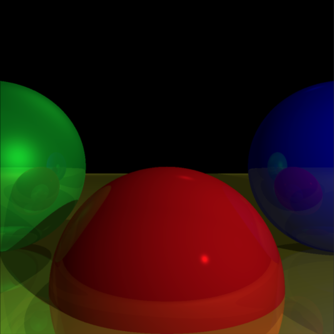
This raytraced scene is just thousands of uses of the quadratic formula.
And to think that we'd never use the quadratic formula in real life.
I Don't Know Where Else to Put This
Before I end off this post, I want to include some other interesting circle facts since I don't know where else to put them.
Squaring the Circle (Bounces)
If you have a ray of light start from the circumference of the circle, after a total of $n$ reflections within the circle, the sum of all the angles of reflection will be $n^2$ times the initial angle.
Between this and the Basel problem, circles and squares are just weirdly intertwined. The reason this particular statement is true is because of how much the angle with the horizontal increases after a single bounce. If your light starts at an angle $\alpha$, we can show that every additional bounce will add $2\alpha$ to the angle with respect to the horizontal.
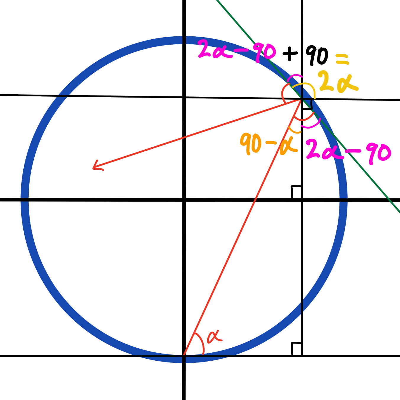
With the help of some auxiliary lines, I hope the above picture makes this clear. Then by symmetry, of the circle, we can see that each subsequent bounce will also add $2\alpha$ to the angle. Moreover, since our initial angle itself is $\alpha$, every bounce will just be the odd multiples of $\alpha$ (since odd numbers can be thought of as a multiple of 2 plus 1, which is precisely what our angle bounces mimic)! So, for a series of $n$ bounces, the sum of the angles of each reflection is equal to
(Yes I am aware there is a formula for an arithmetic sequence with with any initial term but this is how I remember to solve them okay) I didn't know how to fit it in last post with the mention of circular mirrors there, but here seems like a good spot to mention it.
Perpendicular Parabolas
The set of intersection points between two orthogonal parabolas lie on a common circle.
To show this is true, we just need to crank out the algebra. To find our intersection points, we need to solve the system of equations
If these individual equations are true for our intersection points, then so is their sum.
$x^2 - x(2\color{red}{x_1}) + \color{red}{x_1}^2 + y^2 - y(2\color{blue}{y_2}) + \color{blue}{y_2}^2 = y - \color{red}{y_1} + x - \color{blue}{x_2}$
$x^2 - x(2\color{red}{x_1} + 1) + y^2 - y(2\color{blue}{y_2} + 1) = -\color{red}{y_1} - \color{red}{x_1}^2 - \color{blue}{x_2} - \color{blue}{y_2}^2$
$(x - (\color{red}{x_1} + \frac{1}{2}))^2 - (\color{red}{x_1} + \frac{1}{2})^2 + (y - (\color{blue}{y_2} + \frac{1}{2}))^2 - (\color{blue}{y_2} + \frac{1}{2})^2 = -\color{red}{y_1} - \color{red}{x_1}^2 - \color{blue}{x_2} - \color{blue}{y_2}^2$
$(x - (\color{red}{x_1} + \frac{1}{2}))^2 + (y - (\color{blue}{y_2} + \frac{1}{2}))^2 = (\color{red}{x_1} + \frac{1}{2})^2 + (\color{blue}{y_2} + \frac{1}{2})^2 -\color{red}{y_1} - \color{red}{x_1}^2 - \color{blue}{x_2} - \color{blue}{y_2}^2$
While that last line may seem a bit unruly, note that $\color{red}{x_1}$, $\color{red}{y_1}$, $\color{blue}{x_2}$, and $\color{blue}{y_2}$ are all constants, so the right-hand side of that last equation can be summarized as one big constant.
That's precisely the equation of a circle with a center at $(\color{red}{x_1} + \frac{1}{2}, \color{blue}{y_2} + \frac{1}{2})$ and radius $\sqrt{C}$, and that's exactly what is plotted above.
I have a few more circle tidbits to share, but they have more to expand on in their own posts for another day.
Until then, hopefully you found this slight detour into the world of graphics interesting. There are (as you could imagine) a lot more to graphics I want to share. From image homography, to video textures, to even a more in-depth look into raytracing and rasterization, but we'll save those for later.